Tutorial 8: Diff_Tech_MOSTA_integration
This tutorial primarily describes the process of using samples seqFISH(E8.5) and Stereo-seq(E10.5) to interpolate the intermediate data.
Environment Configuration & Package Loading
[1]:
import os
import torch
import scanpy as sc
from GenOT import genot
import warnings

warnings.filterwarnings("ignore")
C:\ProgramData\anaconda3\envs\pytorch\lib\site-packages\scipy\__init__.py:177: UserWarning: A NumPy version >=1.18.5 and <1.26.0 is required for this version of SciPy (detected version 1.26.4
  warnings.warn(f"A NumPy version >={np_minversion} and <{np_maxversion}"
[2]:
# Run device, by default, the package is implemented on 'cpu'. We recommend using GPU.
device = torch.device('cuda:0' if torch.cuda.is_available() else 'cpu')

# the location of R, which is necessary for mclust algorithm. Please replace the path below with local R installation path
os.environ['R_HOME'] = 'C:/Program Files/R/R-4.4.1'
os.environ['PATH'] = 'C:/Program Files/R/R-4.4.1/bin/x64;' + os.environ['PATH']
Data Loading
[3]:
adata1 = sc.read_h5ad(r"..\Data\seqFISH(embryo1).h5ad")
adata1 = sc.pp.subsample(adata1, n_obs=5000, random_state=0, copy=True)
adata2 = sc.read_h5ad(r'..\Data\E10.5_E2S1.MOSTA.h5ad')
adata2 = sc.pp.subsample(adata2, n_obs=5000, random_state=0, copy=True)
[4]:
adata1
[4]:
AnnData object with n_obs × n_vars = 5000 × 351
    obs: 'x_global', 'y_global'
    obsm: 'spatial'
normalize
[5]:
from GenOT.utils import normalize_sparse

adata1 = normalize_sparse(adata1)
adata2 = normalize_sparse(adata2)
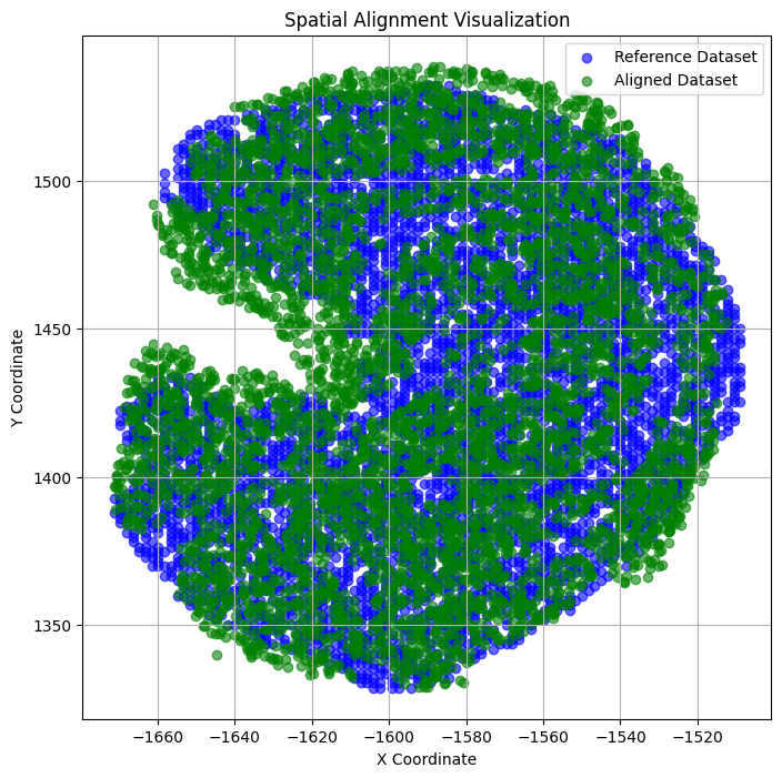
Align the input datasets adata1 and adata2 using the GenOT algorithm.
[6]:
from GenOT.utils import align_spatial_coords
from GenOT.plotting import visualize_alignment

adata2.obsm['spatial'] = align_spatial_coords(adata1.obsm['spatial'], adata2.obsm['spatial'])
Data Preprocessing
[7]:
from GenOT.utils import get_unique_marker_genes

unique_marker_genes = get_unique_marker_genes(adata2, annotation_column_name='annotation', n_top_genes=500)

common_genes = set(unique_marker_genes) & set(adata1.var_names) & set(adata2.var_names)
matching_genes = list(common_genes)

adata1 = adata1[:, matching_genes].copy()
adata2 = adata2[:, matching_genes].copy()
Using annotation column 'annotation' for marker gene analysis...
Unique values in annotation column: ['Mucosal epithelium', 'Cavity', 'Jaw and tooth', 'Spinal cord', 'Dermomyotome', 'Mesenchyme', 'Urogenital ridge', 'Dorsal root ganglion', 'Lung primordium', 'Blood vessel', 'Heart', 'Brain', 'Liver', 'Connective tissue', 'Sclerotome', 'Head mesenchyme', 'Notochord', 'Choroid plexus']
Extracted 2725 unique marker genes from the top 500 genes per annotation group.
First 10 extracted marker genes: ['0610009B22Rik', '0610010K14Rik', '1110004F10Rik', '1110008F13Rik', '1110059E24Rik', '1500011K16Rik', '1700007G11Rik', '1700016D06Rik', '1700020I14Rik', '1700030K09Rik']...
Run GenOT
[8]:
# define model
Encoder = genot.DualEncoder(adata1, adata2, device=device, pca_n=16)
WARNING: adata.X seems to be already log-transformed.
WARNING: adata.X seems to be already log-transformed.
[9]:
adata1, adata2 = Encoder.train_encoder()
Training DualEncoder on 2 datasets with 700 epochs...
Training: 100%|██████████| 700/700 [00:22<00:00, 31.73it/s]
Training completed!
Compute the spatial barycenter
[10]:
from GenOT.OTutils import compute_spatial_barycenter, compute_emb_barycenter

Xb_s, s_transport_plans = compute_spatial_barycenter(adata1, adata2, weight1=0.5, num_barycenters=5000)
It.  |Loss        |Relative loss|Absolute loss
------------------------------------------------
    0|2.314898e+06|0.000000e+00|0.000000e+00
    1|2.314771e+06|5.462569e-05|1.264460e+02
    2|2.314771e+06|3.425678e-08|7.929660e-02
It.  |Loss        |Relative loss|Absolute loss
------------------------------------------------
    0|2.294781e+06|0.000000e+00|0.000000e+00
    1|2.294662e+06|5.172006e-05|1.186801e+02
    2|2.294662e+06|0.000000e+00|0.000000e+00
It.  |Err
-------------------
    0|4.675275e+05|
    0|1.516650e+05|
It.  |Loss        |Relative loss|Absolute loss
------------------------------------------------
    0|6.572961e+03|0.000000e+00|0.000000e+00
    1|1.024273e+02|6.317195e+01|6.470533e+03
    2|8.603164e+01|1.905772e-01|1.639567e+01
    3|8.491370e+01|1.316568e-02|1.117946e+00
    4|8.491370e+01|0.000000e+00|0.000000e+00
It.  |Loss        |Relative loss|Absolute loss
------------------------------------------------
    0|6.088309e+03|0.000000e+00|0.000000e+00
    1|1.051930e+02|5.687753e+01|5.983116e+03
    2|8.100981e+01|2.985213e-01|2.418316e+01
    3|8.026488e+01|9.280841e-03|7.449256e-01
    4|8.026488e+01|0.000000e+00|0.000000e+00
    1|1.438797e+04|
    1|1.926238e+02|
It.  |Loss        |Relative loss|Absolute loss
------------------------------------------------
    0|6.616955e+03|0.000000e+00|0.000000e+00
    1|9.209464e+01|7.084951e+01|6.524860e+03
    2|7.974223e+01|1.549043e-01|1.235242e+01
    3|7.974223e+01|0.000000e+00|0.000000e+00
It.  |Loss        |Relative loss|Absolute loss
------------------------------------------------
    0|6.132303e+03|0.000000e+00|0.000000e+00
    1|1.020939e+02|5.906531e+01|6.030209e+03
    2|8.113876e+01|2.582633e-01|2.095517e+01
    3|8.030877e+01|1.033490e-02|8.299828e-01
    4|8.030877e+01|0.000000e+00|0.000000e+00
    2|1.189078e+04|
    2|1.717228e+02|
It.  |Loss        |Relative loss|Absolute loss
------------------------------------------------
    0|6.617445e+03|0.000000e+00|0.000000e+00
    1|9.759337e+01|6.680630e+01|6.519851e+03
    2|7.999971e+01|2.199214e-01|1.759365e+01
    3|7.999971e+01|0.000000e+00|0.000000e+00
It.  |Loss        |Relative loss|Absolute loss
------------------------------------------------
    0|6.132793e+03|0.000000e+00|0.000000e+00
    1|1.046550e+02|5.760011e+01|6.028138e+03
    2|8.080907e+01|2.950895e-01|2.384591e+01
    3|7.884915e+01|2.485658e-02|1.959920e+00
    4|7.884915e+01|0.000000e+00|0.000000e+00
    3|1.154838e+04|
    3|1.663893e+02|
It.  |Loss        |Relative loss|Absolute loss
------------------------------------------------
    0|6.617705e+03|0.000000e+00|0.000000e+00
    1|9.570413e+01|6.814754e+01|6.522001e+03
    2|7.975721e+01|1.999434e-01|1.594693e+01
    3|7.951438e+01|3.053884e-03|2.428277e-01
    4|7.935990e+01|1.946626e-03|1.544840e-01
    5|7.935990e+01|0.000000e+00|0.000000e+00
It.  |Loss        |Relative loss|Absolute loss
------------------------------------------------
    0|6.133053e+03|0.000000e+00|0.000000e+00
    1|1.021531e+02|5.903783e+01|6.030900e+03
    2|8.004025e+01|2.762723e-01|2.211290e+01
    3|7.987460e+01|2.073905e-03|1.656523e-01
    4|7.987460e+01|0.000000e+00|0.000000e+00
    4|1.168729e+04|
    4|1.684623e+02|
It.  |Loss        |Relative loss|Absolute loss
------------------------------------------------
    0|6.617646e+03|0.000000e+00|0.000000e+00
    1|9.497828e+01|6.867536e+01|6.522668e+03
    2|8.007535e+01|1.861114e-01|1.490294e+01
    3|8.007535e+01|0.000000e+00|0.000000e+00
It.  |Loss        |Relative loss|Absolute loss
------------------------------------------------
    0|6.132995e+03|0.000000e+00|0.000000e+00
    1|1.010490e+02|5.969328e+01|6.031946e+03
    2|7.816845e+01|2.927082e-01|2.288055e+01
    3|7.794053e+01|2.924231e-03|2.279161e-01
    4|7.794053e+01|0.000000e+00|0.000000e+00
    5|1.138724e+04|
    5|1.648396e+02|
It.  |Loss        |Relative loss|Absolute loss
------------------------------------------------
    0|6.617996e+03|0.000000e+00|0.000000e+00
    1|9.604802e+01|6.790300e+01|6.521948e+03
    2|7.936163e+01|2.102576e-01|1.668639e+01
    3|7.936163e+01|0.000000e+00|0.000000e+00
It.  |Loss        |Relative loss|Absolute loss
------------------------------------------------
    0|6.133345e+03|0.000000e+00|0.000000e+00
    1|1.032492e+02|5.840330e+01|6.030095e+03
    2|7.968079e+01|2.957856e-01|2.356843e+01
    3|7.968079e+01|0.000000e+00|0.000000e+00
    6|1.154908e+04|
    6|1.662812e+02|
It.  |Loss        |Relative loss|Absolute loss
------------------------------------------------
    0|6.617605e+03|0.000000e+00|0.000000e+00
    1|9.344444e+01|6.981861e+01|6.524160e+03
    2|7.944942e+01|1.761500e-01|1.399502e+01
    3|7.944942e+01|0.000000e+00|0.000000e+00
It.  |Loss        |Relative loss|Absolute loss
------------------------------------------------
    0|6.132953e+03|0.000000e+00|0.000000e+00
    1|1.042844e+02|5.780990e+01|6.028669e+03
    2|7.828665e+01|3.320837e-01|2.599772e+01
    3|7.828665e+01|0.000000e+00|0.000000e+00
    7|1.117067e+04|
    7|1.616602e+02|
It.  |Loss        |Relative loss|Absolute loss
------------------------------------------------
    0|6.617935e+03|0.000000e+00|0.000000e+00
    1|9.228970e+01|7.070827e+01|6.525645e+03
    2|7.853444e+01|1.751493e-01|1.375525e+01
    3|7.853444e+01|0.000000e+00|0.000000e+00
It.  |Loss        |Relative loss|Absolute loss
------------------------------------------------
    0|6.133283e+03|0.000000e+00|0.000000e+00
    1|1.030581e+02|5.851286e+01|6.030225e+03
    2|7.970933e+01|2.929241e-01|2.334878e+01
    3|7.970933e+01|0.000000e+00|0.000000e+00
    8|1.138726e+04|
    8|1.642540e+02|
It.  |Loss        |Relative loss|Absolute loss
------------------------------------------------
    0|6.617863e+03|0.000000e+00|0.000000e+00
    1|9.459269e+01|6.896168e+01|6.523270e+03
    2|7.954160e+01|1.892228e-01|1.505108e+01
    3|7.923312e+01|3.893315e-03|3.084795e-01
    4|7.916157e+01|9.039126e-04|7.155514e-02
    5|7.916157e+01|0.000000e+00|0.000000e+00
It.  |Loss        |Relative loss|Absolute loss
------------------------------------------------
    0|6.133211e+03|0.000000e+00|0.000000e+00
    1|1.035344e+02|5.823838e+01|6.029677e+03
    2|8.173465e+01|2.667140e-01|2.179977e+01
    3|7.978024e+01|2.449733e-02|1.954403e+00
    4|7.959795e+01|2.290206e-03|1.822957e-01
    5|7.947794e+01|1.509930e-03|1.200061e-01
    6|7.947794e+01|0.000000e+00|0.000000e+00
    9|1.154613e+04|
    9|1.671027e+02|
[11]:
visualize_alignment(adata2.obsm['spatial'], Xb_s)
[12]:
decoder = genot.Decoder(
    input_size=adata1.obsm['emb'].shape[1],  # Input dimension
    output_size=adata1.X.shape[1],  # Output dimension
)
# Train the decoder
trained_decoder = decoder.train_decoder(adata1, adata2, decoder, epochs=500, batch_size=2048)
100%|██████████| 500/500 [00:42<00:00, 11.90it/s]
[13]:
embd0 = adata1.obsm['emb']
embd1 = adata2.obsm['emb']
Compute the embedding barycenter for the latent representations.
[14]:
Xb, e_transport_plans = compute_emb_barycenter(adata1, adata2, weight1=0.5, num_barycenters=5000, alpha=0)
It.  |Loss        |Relative loss|Absolute loss
------------------------------------------------
    0|5.208798e+01|0.000000e+00|0.000000e+00
    1|3.749976e+01|3.890219e-01|1.458823e+01
    2|3.749976e+01|0.000000e+00|0.000000e+00
It.  |Loss        |Relative loss|Absolute loss
------------------------------------------------
    0|3.425884e+01|0.000000e+00|0.000000e+00
    1|2.013684e+01|7.013015e-01|1.412200e+01
    2|2.013684e+01|0.000000e+00|0.000000e+00
It.  |Err
-------------------
    0|9.931621e+03|
    0|3.476126e+02|
It.  |Loss        |Relative loss|Absolute loss
------------------------------------------------
    0|1.635861e+01|0.000000e+00|0.000000e+00
    1|5.092606e+00|2.212227e+00|1.126600e+01
    2|5.092606e+00|0.000000e+00|0.000000e+00
It.  |Loss        |Relative loss|Absolute loss
------------------------------------------------
    0|1.511027e+01|0.000000e+00|0.000000e+00
    1|5.145836e+00|1.936407e+00|9.964434e+00
    2|5.145836e+00|0.000000e+00|0.000000e+00
    1|1.546620e+03|
    1|6.013746e+01|
It.  |Loss        |Relative loss|Absolute loss
------------------------------------------------
    0|1.661408e+01|0.000000e+00|0.000000e+00
    1|4.875967e+00|2.407341e+00|1.173811e+01
    2|4.875967e+00|0.000000e+00|0.000000e+00
It.  |Loss        |Relative loss|Absolute loss
------------------------------------------------
    0|1.536574e+01|0.000000e+00|0.000000e+00
    1|4.939618e+00|2.110715e+00|1.042613e+01
    2|4.939618e+00|0.000000e+00|0.000000e+00
    2|1.412061e+03|
    2|5.482252e+01|
It.  |Loss        |Relative loss|Absolute loss
------------------------------------------------
    0|1.670331e+01|0.000000e+00|0.000000e+00
    1|4.758666e+00|2.510082e+00|1.194464e+01
    2|4.758666e+00|0.000000e+00|0.000000e+00
It.  |Loss        |Relative loss|Absolute loss
------------------------------------------------
    0|1.545497e+01|0.000000e+00|0.000000e+00
    1|4.808377e+00|2.214177e+00|1.064660e+01
    2|4.808377e+00|0.000000e+00|0.000000e+00
    3|1.301164e+03|
    3|5.099077e+01|
It.  |Loss        |Relative loss|Absolute loss
------------------------------------------------
    0|1.674649e+01|0.000000e+00|0.000000e+00
    1|4.703780e+00|2.560219e+00|1.204271e+01
    2|4.703780e+00|0.000000e+00|0.000000e+00
It.  |Loss        |Relative loss|Absolute loss
------------------------------------------------
    0|1.549815e+01|0.000000e+00|0.000000e+00
    1|4.751632e+00|2.261648e+00|1.074652e+01
    2|4.751632e+00|0.000000e+00|0.000000e+00
    4|1.248647e+03|
    4|4.931593e+01|
It.  |Loss        |Relative loss|Absolute loss
------------------------------------------------
    0|1.676871e+01|0.000000e+00|0.000000e+00
    1|4.675610e+00|2.586421e+00|1.209310e+01
    2|4.675610e+00|0.000000e+00|0.000000e+00
It.  |Loss        |Relative loss|Absolute loss
------------------------------------------------
    0|1.552037e+01|0.000000e+00|0.000000e+00
    1|4.716476e+00|2.290671e+00|1.080389e+01
    2|4.716476e+00|0.000000e+00|0.000000e+00
    5|1.219895e+03|
    5|4.868128e+01|
It.  |Loss        |Relative loss|Absolute loss
------------------------------------------------
    0|1.678793e+01|0.000000e+00|0.000000e+00
    1|4.639385e+00|2.618568e+00|1.214855e+01
    2|4.639385e+00|0.000000e+00|0.000000e+00
It.  |Loss        |Relative loss|Absolute loss
------------------------------------------------
    0|1.553959e+01|0.000000e+00|0.000000e+00
    1|4.708396e+00|2.300400e+00|1.083120e+01
    2|4.708396e+00|0.000000e+00|0.000000e+00
    6|1.231704e+03|
    6|4.811677e+01|
It.  |Loss        |Relative loss|Absolute loss
------------------------------------------------
    0|1.679915e+01|0.000000e+00|0.000000e+00
    1|4.623788e+00|2.633201e+00|1.217537e+01
    2|4.623788e+00|0.000000e+00|0.000000e+00
It.  |Loss        |Relative loss|Absolute loss
------------------------------------------------
    0|1.555082e+01|0.000000e+00|0.000000e+00
    1|4.705951e+00|2.304501e+00|1.084487e+01
    2|4.705951e+00|0.000000e+00|0.000000e+00
    7|1.214851e+03|
    7|4.830336e+01|
It.  |Loss        |Relative loss|Absolute loss
------------------------------------------------
    0|1.681177e+01|0.000000e+00|0.000000e+00
    1|4.622062e+00|2.637289e+00|1.218971e+01
    2|4.622062e+00|0.000000e+00|0.000000e+00
It.  |Loss        |Relative loss|Absolute loss
------------------------------------------------
    0|1.556344e+01|0.000000e+00|0.000000e+00
    1|4.685884e+00|2.321344e+00|1.087755e+01
    2|4.685884e+00|0.000000e+00|0.000000e+00
    8|1.201148e+03|
    8|4.793409e+01|
It.  |Loss        |Relative loss|Absolute loss
------------------------------------------------
    0|1.681556e+01|0.000000e+00|0.000000e+00
    1|4.614089e+00|2.644395e+00|1.220147e+01
    2|4.614089e+00|0.000000e+00|0.000000e+00
It.  |Loss        |Relative loss|Absolute loss
------------------------------------------------
    0|1.556722e+01|0.000000e+00|0.000000e+00
    1|4.663115e+00|2.338375e+00|1.090411e+01
    2|4.663115e+00|0.000000e+00|0.000000e+00
    9|1.184182e+03|
    9|4.743709e+01|
Since the spatial barycenter and embedding barycenter reside in different spaces (not one-to-one cell correspondences), we align them by constraining the embedding barycenter. Refer to the [update_embedding_barycenter] function for details.
[15]:
from GenOT.OTutils import update_embedding_barycenter

Xb = update_embedding_barycenter(Xb_s, Xb, s_transport_plans, e_transport_plans)
Use the trained decoder to transform the embedding barycenter into gene expression values.
[16]:
new_embedding = torch.tensor(Xb, dtype=torch.float32)
new_embedding = new_embedding.to("cuda" if torch.cuda.is_available() else "cpu")

trained_decoder.eval()
with torch.no_grad():
    reconstructed_features = trained_decoder(new_embedding)

reconstructed_gene_expression = reconstructed_features.cpu().numpy()

print("Reconstructed Features Shape:", reconstructed_gene_expression.shape)
Reconstructed Features Shape: (5000, 41)
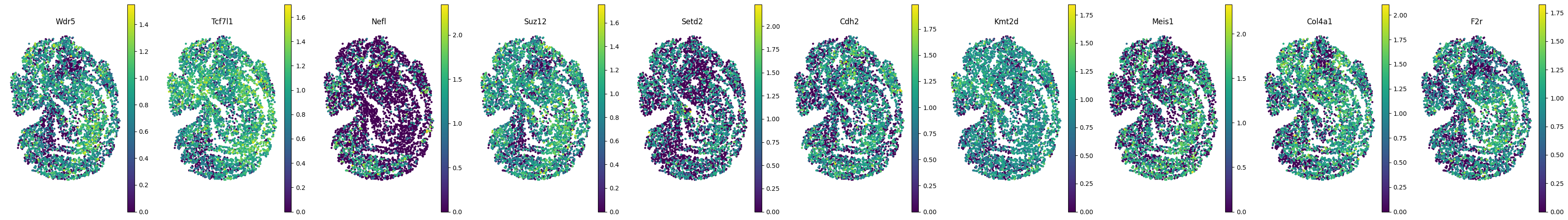
Create a new adata object where the gene expression matrix equals the generated expression values, and spatial coordinates match the spatial barycenter.
[17]:
new_adata = adata1.copy()
X = reconstructed_gene_expression.copy()
thresholds = X.max(axis=0) / 3
for i, threshold in enumerate(thresholds):
    X[:, i][X[:, i] < threshold] = 0
new_adata.X = X
new_adata.obsm['spatial'] = Xb_s
[18]:
import matplotlib.pyplot as plt
import scanpy as sc

common_genes = adata1.var_names
genes_of_interest = list(common_genes)[10:20]

fig, axes = plt.subplots(1, 10, figsize=(35, 5))
plt.subplots_adjust(wspace=0.3)

for i, gene in enumerate(genes_of_interest):
    sc.pl.spatial(
        new_adata,
        color=gene,
        ax=axes[i],
        title=gene,
        show=False,
        size=1.5,
        spot_size=2,
        cmap='viridis',
        frameon=False
    )

plt.tight_layout()
plt.show()
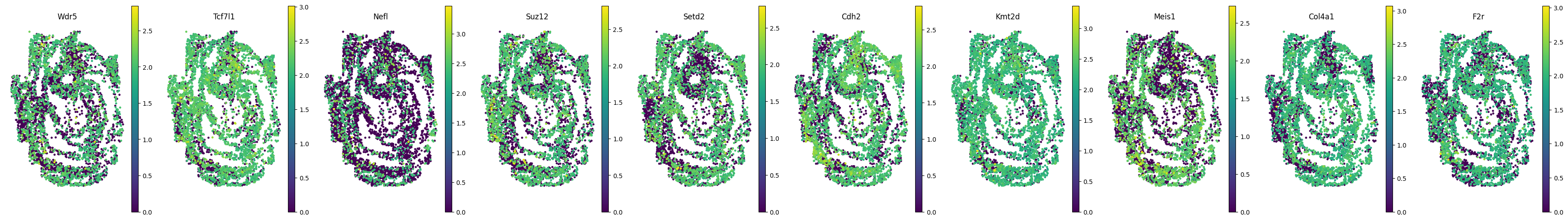
[19]:
common_genes = adata1.var_names
genes_of_interest = list(common_genes)[10:20]

fig, axes = plt.subplots(1, 10, figsize=(35, 5))
plt.subplots_adjust(wspace=0.3)

for i, gene in enumerate(genes_of_interest):
    sc.pl.spatial(
        adata1,
        color=gene,
        ax=axes[i],
        title=gene,
        show=False,
        size=1.5,
        spot_size=2,
        cmap='viridis',
        frameon=False
    )

plt.tight_layout()
plt.show()
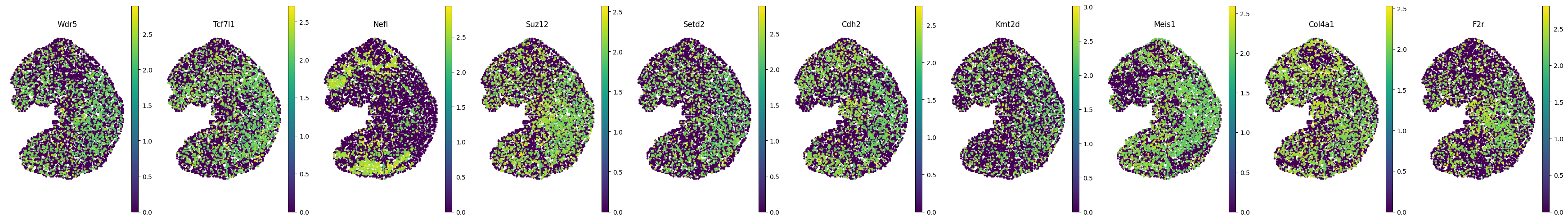
[20]:
common_genes = adata1.var_names
genes_of_interest = list(common_genes)[10:20]

fig, axes = plt.subplots(1, 10, figsize=(35, 5))
plt.subplots_adjust(wspace=0.3)

for i, gene in enumerate(genes_of_interest):
    sc.pl.spatial(
        adata2,
        color=gene,
        ax=axes[i],
        show=False,
        size=1.5,
        spot_size=2,
        cmap='viridis',
        frameon=False
    )

plt.tight_layout()
plt.show()
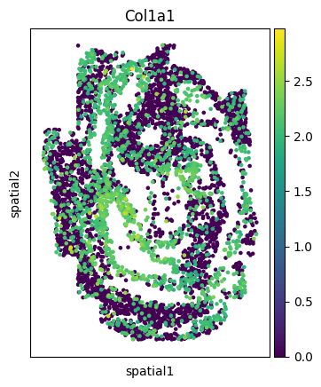
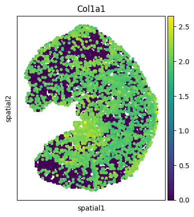
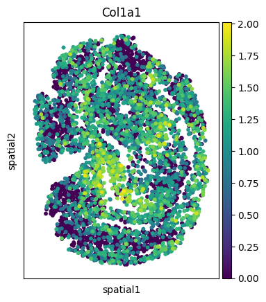
Visualize the Col1a1 gene expression across datasets.
[21]:
sc.pl.spatial(adata1, img_key=None, color='Col1a1', cmap='viridis', size=2, spot_size=1.5)
sc.pl.spatial(adata2, img_key=None, color='Col1a1', cmap='viridis', size=2.5, spot_size=1.5)
sc.pl.spatial(new_adata, img_key=None, color='Col1a1', cmap='viridis', size=2.5, spot_size=1.5)
[21]: