Tutorial 7: MOSTA integration
This tutorial primarily describes the process of using samples E11.5_E1S1 and E11.5_E1S3 to impute E11.5_E1S2.
Environment Configuration & Package Loading
[1]:
import os
import torch
import scanpy as sc
from GenOT import genot
import warnings
warnings.filterwarnings("ignore")
# Run device, by default, the package is implemented on 'cpu'. We recommend using GPU.
device = torch.device('cuda:0' if torch.cuda.is_available() else 'cpu')
# the location of R, which is necessary for mclust algorithm. Please replace the path below with local R installation path
os.environ['R_HOME'] = 'C:/Program Files/R/R-4.4.1'
os.environ['PATH'] = 'C:/Program Files/R/R-4.4.1/bin/x64;' + os.environ['PATH']
C:\ProgramData\anaconda3\envs\pytorch\lib\site-packages\scipy\__init__.py:177: UserWarning: A NumPy version >=1.18.5 and <1.26.0 is required for this version of SciPy (detected version 1.26.4
  warnings.warn(f"A NumPy version >={np_minversion} and <{np_maxversion}"
[1]:
Data Loading
[2]:
adata1 = sc.read_h5ad(r'..\Data\E11.5_E1S1.MOSTA.h5ad')
adata1 = sc.pp.subsample(adata1, n_obs=5000, random_state=0, copy=True)
adata2 = sc.read_h5ad(r'..\Data\E11.5_E1S3.MOSTA.h5ad')
adata2 = sc.pp.subsample(adata2, n_obs=5000, random_state=0, copy=True)
adata3 = sc.read_h5ad(r'..\Data\E11.5_E1S2.MOSTA.h5ad')
adata3 = sc.pp.subsample(adata3, n_obs=5000, random_state=0, copy=True)
normalize
[3]:
from GenOT.utils import normalize_sparse

adata1 = normalize_sparse(adata1)
adata2 = normalize_sparse(adata2)
adata3 = normalize_sparse(adata3)
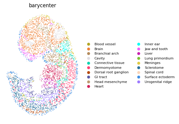
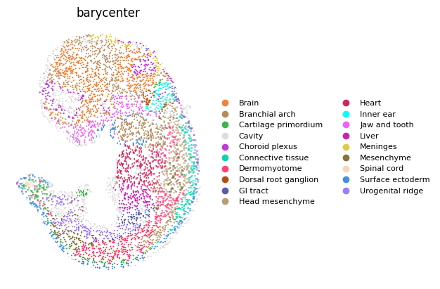
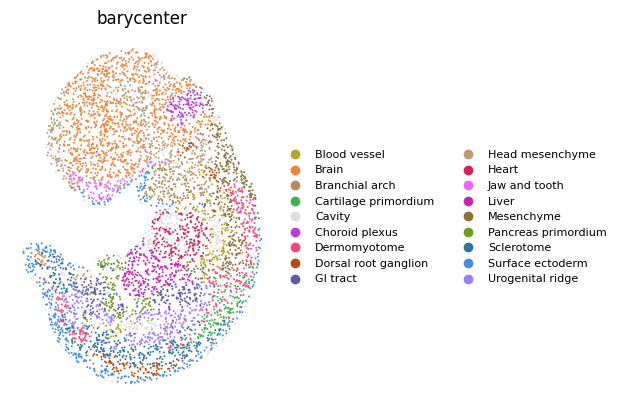
Visualize adata1, adata2, and adata3.
[4]:
sc.pl.spatial(adata1, img_key=None, color='annotation', title='barycenter', size=1.5, legend_fontsize=8,
              show=False, frameon=False, spot_size=1)
sc.pl.spatial(adata2, img_key=None, color='annotation', title='barycenter', size=1.5, legend_fontsize=8,
              show=False, frameon=False, spot_size=1)
sc.pl.spatial(adata3, img_key=None, color='annotation', title='barycenter', size=1.5, legend_fontsize=8,
              show=False, frameon=False, spot_size=1)
[4]:
[<AxesSubplot: title={'center': 'barycenter'}, xlabel='spatial1', ylabel='spatial2'>]
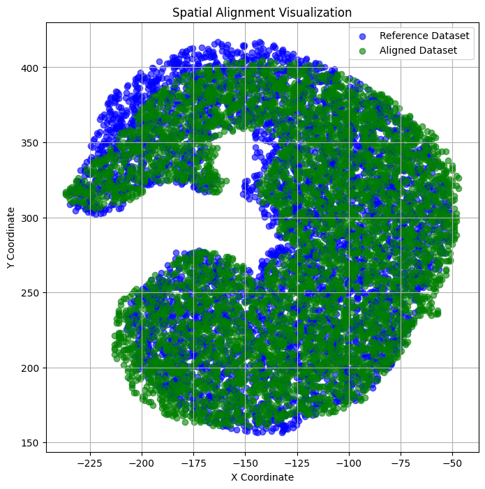
Align the input datasets adata1 and adata2 using the GenOT algorithm.
[5]:
from GenOT.utils import align_spatial_coords
from GenOT.plotting import visualize_alignment
adata2.obsm['spatial']=align_spatial_coords(adata1.obsm['spatial'], adata2.obsm['spatial'],area_ratio_threshold=1)
visualize_alignment(adata1.obsm['spatial'], adata2.obsm['spatial'])
Get unique marker genes from adata3 based on its annotations. These marker genes will be used to ensure consistent gene sets across all datasets.
[6]:
from GenOT.utils import get_unique_marker_genes


unique_marker_genes = get_unique_marker_genes(adata3, annotation_column_name='annotation', n_top_genes= 10)
Using annotation column 'annotation' for marker gene analysis...
Unique values in annotation column: ['Brain', 'Head mesenchyme', 'Cavity', 'Sclerotome', 'Dorsal root ganglion', 'Mesenchyme', 'Dermomyotome', 'Urogenital ridge', 'Heart', 'Branchial arch', 'Blood vessel', 'Surface ectoderm', 'Liver', 'GI tract', 'Choroid plexus', 'Jaw and tooth', 'Pancreas primordium', 'Cartilage primordium']
Extracted 114 unique marker genes from the top 10 genes per annotation group.
First 10 extracted marker genes: ['Acta2', 'Actc1', 'Afp', 'Amot', 'Apex2', 'Apoa2', 'Apoe', 'Asxl3', 'Atp2a2', 'Bc1']...
Data Preprocessing
[7]:
common_genes = set(unique_marker_genes) & set(adata1.var_names) & set(adata2.var_names) & set(adata3.var_names)
matching_genes = list(common_genes)

adata1 = adata1[:, matching_genes].copy()
adata2 = adata2[:, matching_genes].copy()
adata3 = adata3[:, matching_genes].copy()
Run GenOT
[8]:
# define model
Encoder = genot.DualEncoder(adata1,adata2, device=device, pca_n=16)
WARNING: adata.X seems to be already log-transformed.
WARNING: adata.X seems to be already log-transformed.
[9]:
adata1,adata2 = Encoder.train_encoder()
Training DualEncoder on 2 datasets with 700 epochs...
Training: 100%|██████████| 700/700 [00:21<00:00, 31.89it/s]
Training completed!
Compute the spatial barycenter
[10]:
from GenOT.OTutils import compute_spatial_barycenter, compute_emb_barycenter

Xb_s,s_transport_plans=compute_spatial_barycenter(adata1,adata2, weight1=0.5,num_barycenters=adata3.n_obs)
It.  |Loss        |Relative loss|Absolute loss
------------------------------------------------
    0|6.121426e+04|0.000000e+00|0.000000e+00
    1|6.106914e+04|2.376419e-03|1.451259e+02
    2|6.106905e+04|1.395421e-06|8.521707e-02
It.  |Loss        |Relative loss|Absolute loss
------------------------------------------------
    0|5.810448e+04|0.000000e+00|0.000000e+00
    1|5.796061e+04|2.482145e-03|1.438666e+02
    2|5.796061e+04|0.000000e+00|0.000000e+00
It.  |Err
-------------------
    0|5.612321e+05|
    0|2.304730e+04|
It.  |Loss        |Relative loss|Absolute loss
------------------------------------------------
    0|9.203229e+03|0.000000e+00|0.000000e+00
    1|8.424181e+01|1.082478e+02|9.118987e+03
    2|3.998680e+01|1.106741e+00|4.425501e+01
    3|3.998680e+01|0.000000e+00|0.000000e+00
It.  |Loss        |Relative loss|Absolute loss
------------------------------------------------
    0|9.070789e+03|0.000000e+00|0.000000e+00
    1|8.017388e+01|1.121390e+02|8.990616e+03
    2|4.125798e+01|9.432334e-01|3.891590e+01
    3|4.100101e+01|6.267417e-03|2.569704e-01
    4|4.019505e+01|2.005125e-02|8.059610e-01
    5|3.984684e+01|8.738687e-03|3.482091e-01
    6|3.984684e+01|0.000000e+00|0.000000e+00
    1|1.427466e+04|
    1|1.817036e+02|
It.  |Loss        |Relative loss|Absolute loss
------------------------------------------------
    0|9.268094e+03|0.000000e+00|0.000000e+00
    1|7.510326e+01|1.224047e+02|9.192991e+03
    2|3.366767e+01|1.230724e+00|4.143559e+01
    3|3.366767e+01|0.000000e+00|0.000000e+00
It.  |Loss        |Relative loss|Absolute loss
------------------------------------------------
    0|9.135654e+03|0.000000e+00|0.000000e+00
    1|7.363237e+01|1.230712e+02|9.062022e+03
    2|3.413439e+01|1.157132e+00|3.949798e+01
    3|3.413439e+01|0.000000e+00|0.000000e+00
    2|7.710250e+03|
    2|1.123435e+02|
It.  |Loss        |Relative loss|Absolute loss
------------------------------------------------
    0|9.269184e+03|0.000000e+00|0.000000e+00
    1|7.518557e+01|1.222841e+02|9.193998e+03
    2|3.408859e+01|1.205594e+00|4.109698e+01
    3|3.353602e+01|1.647688e-02|5.525689e-01
    4|3.353602e+01|0.000000e+00|0.000000e+00
It.  |Loss        |Relative loss|Absolute loss
------------------------------------------------
    0|9.136744e+03|0.000000e+00|0.000000e+00
    1|7.192908e+01|1.260243e+02|9.064815e+03
    2|3.394929e+01|1.118721e+00|3.797979e+01
    3|3.394929e+01|0.000000e+00|0.000000e+00
    3|7.594237e+03|
    3|1.103562e+02|
It.  |Loss        |Relative loss|Absolute loss
------------------------------------------------
    0|9.269262e+03|0.000000e+00|0.000000e+00
    1|7.290056e+01|1.261494e+02|9.196362e+03
    2|3.335169e+01|1.185813e+00|3.954887e+01
    3|3.262053e+01|2.241434e-02|7.311675e-01
    4|3.262053e+01|0.000000e+00|0.000000e+00
It.  |Loss        |Relative loss|Absolute loss
------------------------------------------------
    0|9.136823e+03|0.000000e+00|0.000000e+00
    1|7.456546e+01|1.215343e+02|9.062257e+03
    2|3.395795e+01|1.195818e+00|4.060751e+01
    3|3.317430e+01|2.362205e-02|7.836450e-01
    4|3.317430e+01|0.000000e+00|0.000000e+00
    4|6.942204e+03|
    4|1.006905e+02|
It.  |Loss        |Relative loss|Absolute loss
------------------------------------------------
    0|9.269714e+03|0.000000e+00|0.000000e+00
    1|7.001124e+01|1.314032e+02|9.199703e+03
    2|3.354127e+01|1.087316e+00|3.646997e+01
    3|3.341978e+01|3.635301e-03|1.214910e-01
    4|3.223502e+01|3.675388e-02|1.184762e+00
    5|3.223502e+01|0.000000e+00|0.000000e+00
It.  |Loss        |Relative loss|Absolute loss
------------------------------------------------
    0|9.137275e+03|0.000000e+00|0.000000e+00
    1|7.142630e+01|1.269259e+02|9.065848e+03
    2|3.309088e+01|1.158489e+00|3.833542e+01
    3|3.252906e+01|1.727118e-02|5.618152e-01
    4|3.252906e+01|0.000000e+00|0.000000e+00
    5|6.460534e+03|
    5|9.357399e+01|
It.  |Loss        |Relative loss|Absolute loss
------------------------------------------------
    0|9.269962e+03|0.000000e+00|0.000000e+00
    1|7.633550e+01|1.204371e+02|9.193627e+03
    2|3.326579e+01|1.294715e+00|4.306971e+01
    3|3.230034e+01|2.988972e-02|9.654482e-01
    4|3.214044e+01|4.975128e-03|1.599028e-01
    5|3.214044e+01|0.000000e+00|0.000000e+00
It.  |Loss        |Relative loss|Absolute loss
------------------------------------------------
    0|9.137523e+03|0.000000e+00|0.000000e+00
    1|7.199068e+01|1.259265e+02|9.065532e+03
    2|3.389566e+01|1.123891e+00|3.809502e+01
    3|3.351240e+01|1.143644e-02|3.832626e-01
    4|3.351240e+01|0.000000e+00|0.000000e+00
    6|7.063295e+03|
    6|1.027254e+02|
It.  |Loss        |Relative loss|Absolute loss
------------------------------------------------
    0|9.269860e+03|0.000000e+00|0.000000e+00
    1|7.159322e+01|1.284796e+02|9.198267e+03
    2|3.326715e+01|1.152070e+00|3.832607e+01
    3|3.212530e+01|3.554371e-02|1.141852e+00
    4|3.212530e+01|0.000000e+00|0.000000e+00
It.  |Loss        |Relative loss|Absolute loss
------------------------------------------------
    0|9.137421e+03|0.000000e+00|0.000000e+00
    1|7.303599e+01|1.241085e+02|9.064385e+03
    2|3.279640e+01|1.226951e+00|4.023958e+01
    3|3.277504e+01|6.519256e-04|2.136689e-02
    4|3.277504e+01|0.000000e+00|0.000000e+00
    7|6.784982e+03|
    7|9.858325e+01|
It.  |Loss        |Relative loss|Absolute loss
------------------------------------------------
    0|9.270076e+03|0.000000e+00|0.000000e+00
    1|7.238577e+01|1.270649e+02|9.197690e+03
    2|3.346771e+01|1.162854e+00|3.891805e+01
    3|3.293349e+01|1.622116e-02|5.342194e-01
    4|3.234216e+01|1.828357e-02|5.913302e-01
    5|3.234216e+01|0.000000e+00|0.000000e+00
It.  |Loss        |Relative loss|Absolute loss
------------------------------------------------
    0|9.137637e+03|0.000000e+00|0.000000e+00
    1|7.341996e+01|1.234571e+02|9.064217e+03
    2|3.314441e+01|1.215154e+00|4.027555e+01
    3|3.314441e+01|0.000000e+00|0.000000e+00
    8|7.034249e+03|
    8|1.025523e+02|
It.  |Loss        |Relative loss|Absolute loss
------------------------------------------------
    0|9.269932e+03|0.000000e+00|0.000000e+00
    1|7.382425e+01|1.245676e+02|9.196108e+03
    2|3.321296e+01|1.222754e+00|4.061129e+01
    3|3.277893e+01|1.324121e-02|4.340327e-01
    4|3.269873e+01|2.452680e-03|8.019950e-02
    5|3.269873e+01|0.000000e+00|0.000000e+00
It.  |Loss        |Relative loss|Absolute loss
------------------------------------------------
    0|9.137492e+03|0.000000e+00|0.000000e+00
    1|6.704690e+01|1.352851e+02|9.070445e+03
    2|3.314351e+01|1.022927e+00|3.390340e+01
    3|3.314351e+01|0.000000e+00|0.000000e+00
    9|7.428341e+03|
    9|1.082719e+02|
[11]:
decoder = genot.Decoder(
    input_size=adata1.obsm['emb'].shape[1],  # Input dimension
    output_size=adata1.X.shape[1],  # Output dimension
)
# Train the decoder
trained_decoder = decoder.train_decoder(adata1, adata2, decoder, epochs=500, batch_size=2048)
100%|██████████| 500/500 [01:04<00:00, 7.75it/s]
[12]:
embd0 = adata1.obsm['emb']
embd1 = adata2.obsm['emb']
Compute the embedding barycenter for the latent representations.
[13]:
Xb,e_transport_plans = compute_emb_barycenter(adata1, adata2, weight1=0.5, num_barycenters=adata3.n_obs)
It.  |Loss        |Relative loss|Absolute loss
------------------------------------------------
    0|1.425957e+02|0.000000e+00|0.000000e+00
    1|1.338667e+02|6.520663e-02|8.728996e+00
    2|1.338618e+02|3.666998e-05|4.908709e-03
    3|1.338618e+02|0.000000e+00|0.000000e+00
It.  |Loss        |Relative loss|Absolute loss
------------------------------------------------
    0|6.418874e+01|0.000000e+00|0.000000e+00
    1|5.432863e+01|1.814901e-01|9.860108e+00
    2|5.432863e+01|0.000000e+00|0.000000e+00
It.  |Err
-------------------
    0|7.157228e+03|
    0|9.267090e+02|
It.  |Loss        |Relative loss|Absolute loss
------------------------------------------------
    0|2.161672e+01|0.000000e+00|0.000000e+00
    1|7.224797e+00|1.992018e+00|1.439192e+01
    2|7.224797e+00|0.000000e+00|0.000000e+00
It.  |Loss        |Relative loss|Absolute loss
------------------------------------------------
    0|2.453813e+01|0.000000e+00|0.000000e+00
    1|7.535333e+00|2.256410e+00|1.700280e+01
    2|7.456074e+00|1.063018e-02|7.925942e-02
    3|7.456074e+00|0.000000e+00|0.000000e+00
    1|2.403458e+03|
    1|7.725738e+01|
It.  |Loss        |Relative loss|Absolute loss
------------------------------------------------
    0|2.218043e+01|0.000000e+00|0.000000e+00
    1|7.101454e+00|2.123364e+00|1.507897e+01
    2|7.083599e+00|2.520518e-03|1.785434e-02
    3|7.061807e+00|3.085977e-03|2.179257e-02
    4|7.061807e+00|0.000000e+00|0.000000e+00
It.  |Loss        |Relative loss|Absolute loss
------------------------------------------------
    0|2.510184e+01|0.000000e+00|0.000000e+00
    1|7.202467e+00|2.485173e+00|1.789937e+01
    2|7.127214e+00|1.055852e-02|7.525280e-02
    3|7.127214e+00|0.000000e+00|0.000000e+00
    2|1.932257e+03|
    2|6.805194e+01|
It.  |Loss        |Relative loss|Absolute loss
------------------------------------------------
    0|2.225173e+01|0.000000e+00|0.000000e+00
    1|7.054785e+00|2.154132e+00|1.519694e+01
    2|7.046922e+00|1.115855e-03|7.863340e-03
    3|7.040260e+00|9.462185e-04|6.661625e-03
    4|7.036713e+00|5.041681e-04|3.547686e-03
    5|6.997589e+00|5.591040e-03|3.912380e-02
    6|6.997589e+00|0.000000e+00|0.000000e+00
It.  |Loss        |Relative loss|Absolute loss
------------------------------------------------
    0|2.517314e+01|0.000000e+00|0.000000e+00
    1|7.146212e+00|2.522585e+00|1.802693e+01
    2|7.095289e+00|7.177137e-03|5.092386e-02
    3|7.067100e+00|3.988772e-03|2.818905e-02
    4|7.067100e+00|0.000000e+00|0.000000e+00
    3|1.849426e+03|
    3|6.573352e+01|
It.  |Loss        |Relative loss|Absolute loss
------------------------------------------------
    0|2.227661e+01|0.000000e+00|0.000000e+00
    1|7.041734e+00|2.163512e+00|1.523488e+01
    2|7.007703e+00|4.856317e-03|3.403163e-02
    3|7.007106e+00|8.508107e-05|5.961721e-04
    4|6.993850e+00|1.895392e-03|1.325609e-02
    5|6.993850e+00|0.000000e+00|0.000000e+00
It.  |Loss        |Relative loss|Absolute loss
------------------------------------------------
    0|2.519802e+01|0.000000e+00|0.000000e+00
    1|7.114085e+00|2.541991e+00|1.808394e+01
    2|7.081187e+00|4.645846e-03|3.289811e-02
    3|7.071046e+00|1.434237e-03|1.014155e-02
    4|7.065981e+00|7.167973e-04|5.064876e-03
    5|7.042018e+00|3.402797e-03|2.396256e-02
    6|7.042018e+00|0.000000e+00|0.000000e+00
    4|1.833266e+03|
    4|6.546897e+01|
It.  |Loss        |Relative loss|Absolute loss
------------------------------------------------
    0|2.228636e+01|0.000000e+00|0.000000e+00
    1|7.012074e+00|2.178283e+00|1.527429e+01
    2|7.012074e+00|0.000000e+00|0.000000e+00
It.  |Loss        |Relative loss|Absolute loss
------------------------------------------------
    0|2.520777e+01|0.000000e+00|0.000000e+00
    1|7.115926e+00|2.542444e+00|1.809185e+01
    2|7.070157e+00|6.473647e-03|4.576970e-02
    3|7.070157e+00|0.000000e+00|0.000000e+00
    5|1.864595e+03|
    5|6.658136e+01|
It.  |Loss        |Relative loss|Absolute loss
------------------------------------------------
    0|2.228018e+01|0.000000e+00|0.000000e+00
    1|7.009660e+00|2.178497e+00|1.527052e+01
    2|6.994432e+00|2.177207e-03|1.522833e-02
    3|6.994432e+00|0.000000e+00|0.000000e+00
It.  |Loss        |Relative loss|Absolute loss
------------------------------------------------
    0|2.520160e+01|0.000000e+00|0.000000e+00
    1|7.098632e+00|2.550205e+00|1.810297e+01
    2|7.045460e+00|7.546959e-03|5.317180e-02
    3|7.042044e+00|4.852065e-04|3.416845e-03
    4|7.042044e+00|0.000000e+00|0.000000e+00
    6|1.835442e+03|
    6|6.575282e+01|
It.  |Loss        |Relative loss|Absolute loss
------------------------------------------------
    0|2.228994e+01|0.000000e+00|0.000000e+00
    1|7.025932e+00|2.172525e+00|1.526401e+01
    2|7.000314e+00|3.659491e-03|2.561758e-02
    3|6.980046e+00|2.903720e-03|2.026810e-02
    4|6.980046e+00|0.000000e+00|0.000000e+00
It.  |Loss        |Relative loss|Absolute loss
------------------------------------------------
    0|2.521135e+01|0.000000e+00|0.000000e+00
    1|7.140122e+00|2.530941e+00|1.807123e+01
    2|7.053410e+00|1.229367e-02|8.671232e-02
    3|7.053410e+00|0.000000e+00|0.000000e+00
    7|1.832101e+03|
    7|6.579283e+01|
It.  |Loss        |Relative loss|Absolute loss
------------------------------------------------
    0|2.229173e+01|0.000000e+00|0.000000e+00
    1|7.021292e+00|2.174876e+00|1.527044e+01
    2|6.997274e+00|3.432530e-03|2.401835e-02
    3|6.985937e+00|1.622822e-03|1.133693e-02
    4|6.981299e+00|6.643524e-04|4.638043e-03
    5|6.981299e+00|0.000000e+00|0.000000e+00
It.  |Loss        |Relative loss|Absolute loss
------------------------------------------------
    0|2.521315e+01|0.000000e+00|0.000000e+00
    1|7.092811e+00|2.554747e+00|1.812033e+01
    2|7.011452e+00|1.160373e-02|8.135897e-02
    3|7.011452e+00|0.000000e+00|0.000000e+00
    8|1.806353e+03|
    8|6.509501e+01|
It.  |Loss        |Relative loss|Absolute loss
------------------------------------------------
    0|2.230108e+01|0.000000e+00|0.000000e+00
    1|7.012374e+00|2.180247e+00|1.528870e+01
    2|7.002710e+00|1.379994e-03|9.663697e-03
    3|6.986263e+00|2.354152e-03|1.644672e-02
    4|6.986263e+00|0.000000e+00|0.000000e+00
It.  |Loss        |Relative loss|Absolute loss
------------------------------------------------
    0|2.522249e+01|0.000000e+00|0.000000e+00
    1|7.102330e+00|2.551298e+00|1.812016e+01
    2|7.044154e+00|8.258807e-03|5.817631e-02
    3|7.044154e+00|0.000000e+00|0.000000e+00
    9|1.830774e+03|
    9|6.578940e+01|
Since the spatial barycenter and embedding barycenter reside in different spaces (not one-to-one cell correspondences), we align them by constraining the embedding barycenter. Refer to the [update_embedding_barycenter] function for details.
[14]:
from GenOT.OTutils import update_embedding_barycenter

Xb = update_embedding_barycenter(Xb_s, Xb, s_transport_plans, e_transport_plans)
Use the trained decoder to transform the embedding barycenter into gene expression values.
[15]:
new_embedding = torch.tensor(Xb, dtype=torch.float32)
new_embedding = new_embedding.to("cuda" if torch.cuda.is_available() else "cpu")

trained_decoder.eval()
with torch.no_grad():
    reconstructed_features = trained_decoder(new_embedding)

reconstructed_gene_expression = reconstructed_features.cpu().numpy()

print("Reconstructed Features Shape:", reconstructed_gene_expression.shape)
Reconstructed Features Shape: (5000, 114)
Create a new adata object where the gene expression matrix equals the generated expression values, and spatial coordinates match the spatial barycenter.
[16]:
new_adata = adata3.copy()
X=reconstructed_gene_expression.copy()
thresholds = X.max(axis=0) /3
for i, threshold in enumerate(thresholds):
        X[:, i][X[:, i] < threshold] = 0
new_adata.X = X
new_adata.obsm['spatial'] = Xb_s
[16]:
[17]:
import matplotlib.pyplot as plt
import scanpy as sc


genes_of_interest = list(common_genes)[:10]

fig, axes = plt.subplots(1, 10, figsize=(35, 5))
plt.subplots_adjust(wspace=0.3)

for i, gene in enumerate(genes_of_interest):
    sc.pl.spatial(
        new_adata,
        color=gene,
        ax=axes[i],
        title=gene,
        show=False,
        size=1.5,
        spot_size=1,
        cmap='viridis',
        frameon=False
    )

plt.tight_layout()
plt.show()
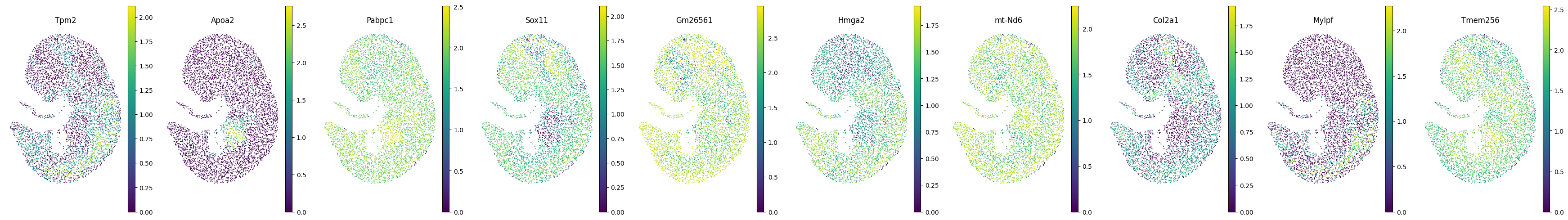
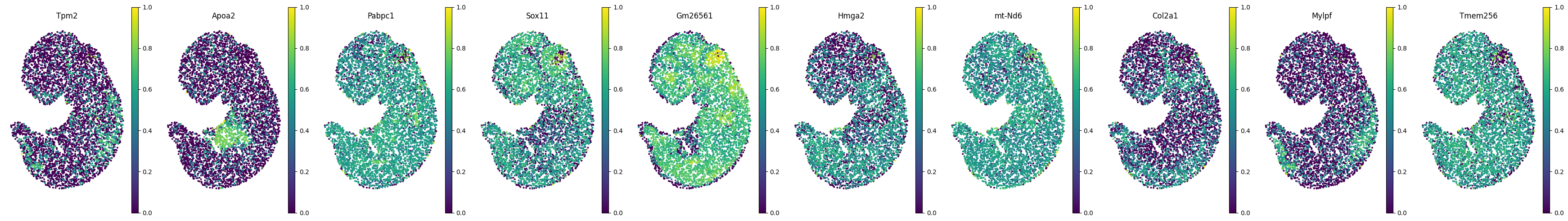
Map the generated gene expression data to the target dataset using the [create_mapped_adata] function.
[18]:
from GenOT.OTutils import create_mapped_adata


mapped_adata = create_mapped_adata(new_adata, adata3,threshold_denominator=3)
Visualize the mapped data, original datasets (adata1 and adata2), and the imputed dataset (adata3)
[19]:
import matplotlib.pyplot as plt
import scanpy as sc


genes_of_interest = list(common_genes)[:10]

fig, axes = plt.subplots(1, 10, figsize=(35, 5))
plt.subplots_adjust(wspace=0.3)

for i, gene in enumerate(genes_of_interest):
    sc.pl.spatial(
        mapped_adata,
        color=gene,
        ax=axes[i],
        title=gene,
        show=False,
        size=1.5,
        spot_size=2,
        cmap='viridis',
        frameon=False
    )

plt.tight_layout()
plt.show()
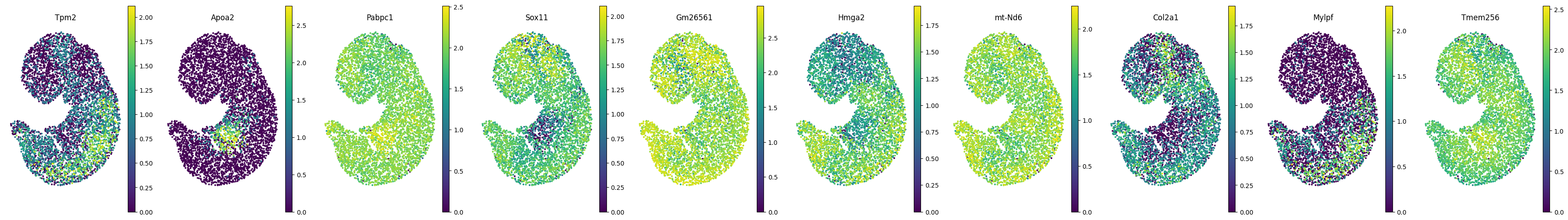
[20]:
genes_of_interest = list(common_genes)[:10]

fig, axes = plt.subplots(1, 10, figsize=(35, 5))
plt.subplots_adjust(wspace=0.3)

for i, gene in enumerate(genes_of_interest):
    sc.pl.spatial(
        adata1,
        color=gene,
        ax=axes[i],
        title=gene,
        show=False,
        size=1.5,
        spot_size=2,
        cmap='viridis',
        frameon=False
    )

plt.tight_layout()
plt.show()
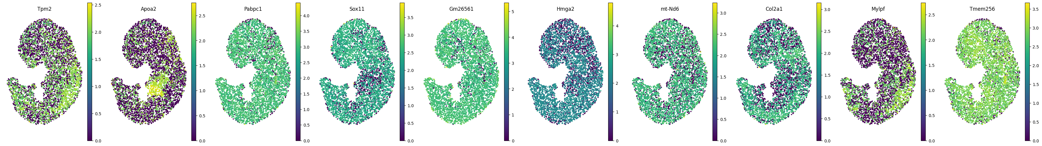
[21]:
genes_of_interest = list(common_genes)[:10]

fig, axes = plt.subplots(1, 10, figsize=(35, 5))
plt.subplots_adjust(wspace=0.3)

for i, gene in enumerate(genes_of_interest):
    sc.pl.spatial(
        adata2,
        color=gene,
        ax=axes[i],
        show=False,
        size=1.5,
        spot_size=2,
        cmap='viridis',
        frameon=False
    )

plt.tight_layout()
plt.show()
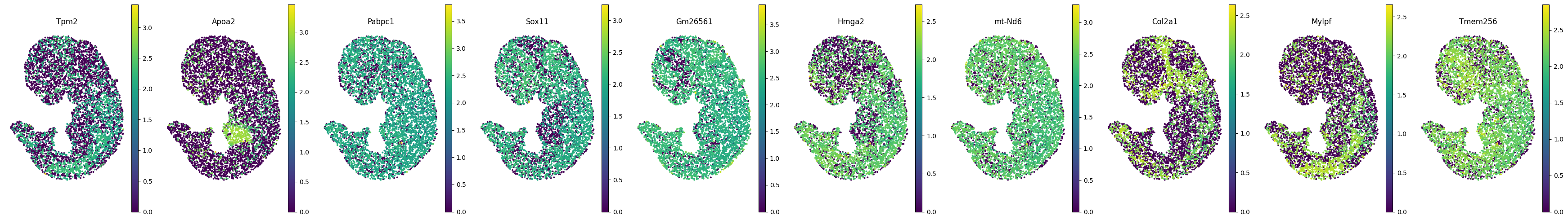
[22]:
common_genes = adata1.var_names
genes_of_interest = list(common_genes)[:10]


fig, axes = plt.subplots(1, 10, figsize=(35, 5))
plt.subplots_adjust(wspace=0.3)

for i, gene in enumerate(genes_of_interest):
    sc.pl.spatial(
        adata3,
        color=gene,
        ax=axes[i],
        title=gene,
        show=False,
        size=1.5,
        spot_size=2,
        cmap='viridis',
        frameon=False
    )

plt.tight_layout()
plt.show()
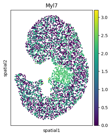
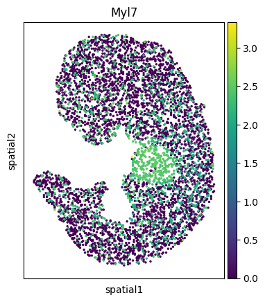
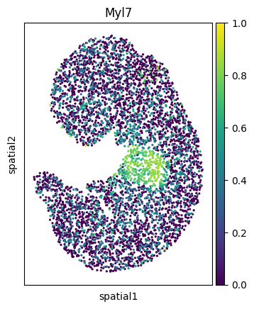
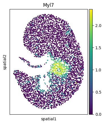
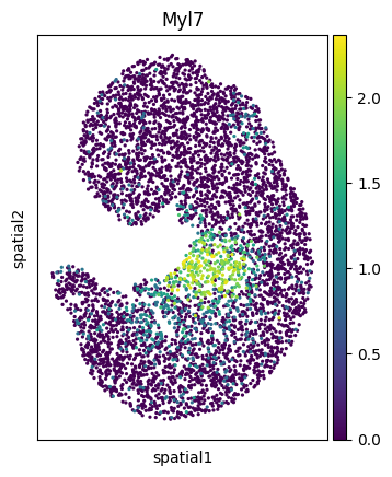
Visualize the Myl7 gene expression across datasets.
[23]:
sc.pl.spatial(adata1, img_key=None, color='Myl7', cmap='viridis', size=2.5, spot_size=1)
sc.pl.spatial(adata2, img_key=None, color='Myl7', cmap='viridis', size=2.5, spot_size=1)
sc.pl.spatial(adata3, img_key=None, color='Myl7', cmap='viridis', size=2.5, spot_size=1)
sc.pl.spatial(new_adata, img_key=None, color='Myl7', cmap='viridis', size=2.5, spot_size=1)
sc.pl.spatial(mapped_adata ,img_key=None, color='Myl7', cmap='viridis', size=2.5, spot_size=1)
[23]:
[24]:
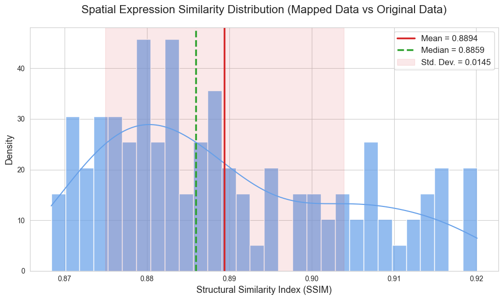
from GenOT.plotting import compare_spatial_expression_all_genes
# Compare the spatial expression patterns between the mapped (imputed) data and the original target data.
# This function calculates and plots similarity metrics (e.g., SSIM) for all genes.
mean_ssim, scores_df = compare_spatial_expression_all_genes(
    adata1=mapped_adata,
    adata1_name="Mapped Data",
    adata2=adata3,
    adata2_name="Original Data",
    max_genes=None,
    output_csv=None,
    plot_file=None,
    figsize=(10, 6)
)
Starting comparison for 114 common genes...
Calculating gene SSIM scores: 100%|██████████| 114/114 [03:32<00:00, 1.86s/it]
==================================================
Analysis complete! Processed 114 genes
Mean SSIM: 0.8894 ± 0.0145
Median SSIM: 0.8859
==================================================
[25]:
from GenOT.plotting import calculate_gene_embedding_metrics, plot_gene_embedding_metrics_distributions
# Calculate various metrics to evaluate the quality of the gene embeddings derived from the imputation.
# These metrics assess how well the imputed gene expression preserves the original's gene-embedding relationships.
df = calculate_gene_embedding_metrics(adata3, mapped_adata, n_pca_components=16)
# Plot the distributions of these calculated gene embedding metrics.
plot_gene_embedding_metrics_distributions(df)
--- Starting gene embedding metric calculation ---
Original adata shape: (5000, 114)
Original mapped_adata shape: (5000, 114)
Transposed adata_g1 shape (genes x cells): (114, 5000)
Transposed adata_g2 shape (genes x cells): (114, 5000)
Found 114 common genes for analysis.
adata_g1 shape after common gene filtering: (114, 5000)
adata_g2 shape after common gene filtering: (114, 5000)

Performing PCA (16 dimensions) for both datasets...
Gene embedding dimensions for Dataset 1: (114, 16)
Gene embedding dimensions for Dataset 2: (114, 16)

Calculating similarity metrics: PCC, Cosine Similarity, RMSE, JS Divergence...

--- Metric calculation complete ---

--- Generating distribution plots for similarity metrics ---
Average PCC: 0.5715
Average Cosine Similarity: 0.5706
Average RMSE: 12.6275
Average JS Divergence: 0.4576
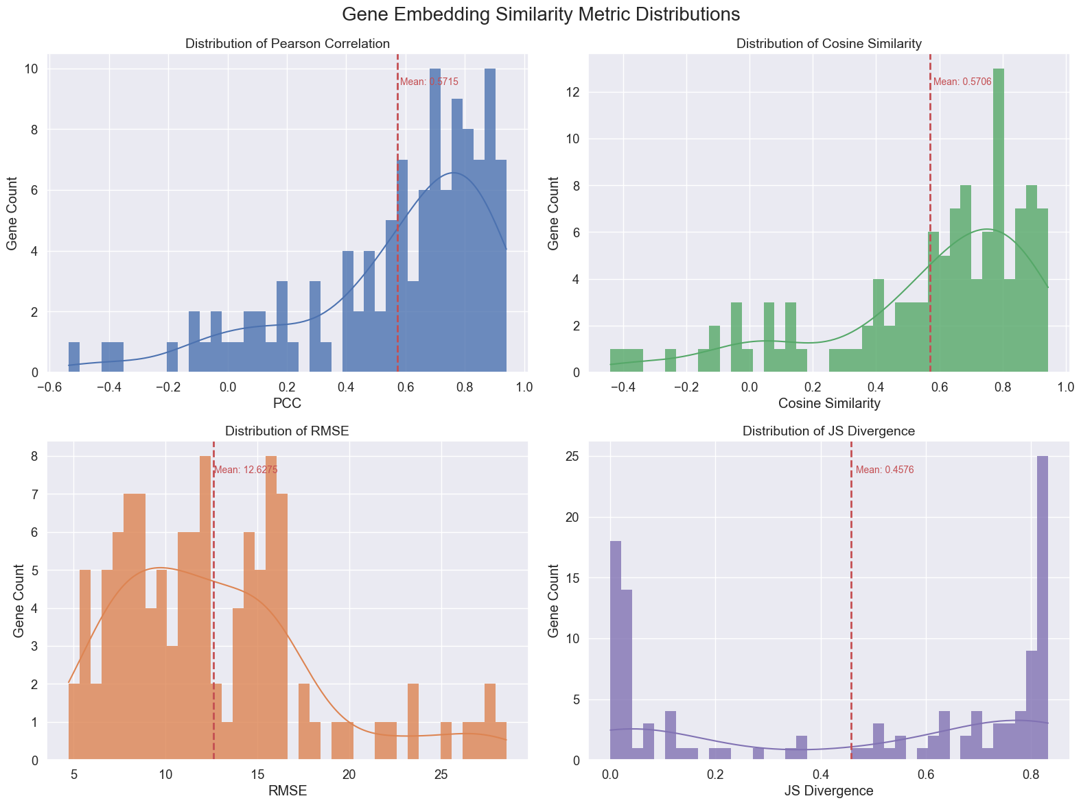
--- Visualization complete ---
[25]:
[25]: