Tutorial 6: DLPFC interpolation

This tutorial primarily describes the process of using samples 151673 and 151675 to impute 151674.

Environment Configuration & Package Loading

[1]:

import os
import torch
import pandas as pd
import scanpy as sc
from GenOT import genot
import warnings

warnings.filterwarnings("ignore")
# Run device, by default, the package is implemented on 'cpu'. We recommend using GPU.
device = torch.device('cuda:0' if torch.cuda.is_available() else 'cpu')

# the location of R, which is necessary for mclust algorithm. Please replace the path below with local R installation path
os.environ['R_HOME'] = 'C:/Program Files/R/R-4.4.1'
os.environ['PATH'] = 'C:/Program Files/R/R-4.4.1/bin/x64;' + os.environ['PATH']

C:\ProgramData\anaconda3\envs\pytorch\lib\site-packages\scipy\__init__.py:177: UserWarning: A NumPy version >=1.18.5 and <1.26.0 is required for this version of SciPy (detected version 1.26.4
  warnings.warn(f"A NumPy version >={np_minversion} and <{np_maxversion}"

Data Loading

We load three different Visium spatial transcriptomics datasets from the DLPFC (Dorsolateral Prefrontal Cortex) region. These datasets will be used for interpolation and analysis.

[2]:

section_id = '151673'
input_dir = os.path.join('../Data', section_id)
adata1 = sc.read_visium(path=input_dir, count_file=section_id + '_filtered_feature_bc_matrix.h5', load_images=True)
adata1.var_names_make_unique(join="++")
print(adata1)
Ann_df = pd.read_csv(os.path.join(input_dir, section_id + '_truth.txt'), sep='\t', header=None, index_col=0)
Ann_df.columns = ['Ground Truth']
Ann_df[Ann_df.isna()] = "unknown"
adata1.obs['Ground Truth'] = Ann_df.loc[adata1.obs_names, 'Ground Truth'].astype('category')

section_id = '151675'
input_dir = os.path.join('../Data', section_id)
adata2 = sc.read_visium(path=input_dir, count_file=section_id + '_filtered_feature_bc_matrix.h5', load_images=True)
adata2.var_names_make_unique(join="++")
print(adata2)
Ann_df = pd.read_csv(os.path.join(input_dir, section_id + '_truth.txt'), sep='\t', header=None, index_col=0)
Ann_df.columns = ['Ground Truth']
Ann_df[Ann_df.isna()] = "unknown"
adata2.obs['Ground Truth'] = Ann_df.loc[adata2.obs_names, 'Ground Truth'].astype('category')

section_id = '151674'
input_dir = os.path.join('../Data', section_id)
adata3 = sc.read_visium(path=input_dir, count_file=section_id + '_filtered_feature_bc_matrix.h5', load_images=True)
# adata3 = sc.pp.subsample(adata3, n_obs=3000, random_state=0, copy=True)
adata3.var_names_make_unique(join="++")
print(adata3)
Ann_df = pd.read_csv(os.path.join(input_dir, section_id + '_truth.txt'), sep='\t', header=None, index_col=0)
Ann_df.columns = ['Ground Truth']
Ann_df[Ann_df.isna()] = "unknown"
adata3.obs['Ground Truth'] = Ann_df.loc[adata3.obs_names, 'Ground Truth'].astype('category')

AnnData object with n_obs × n_vars = 3639 × 33538
    obs: 'in_tissue', 'array_row', 'array_col'
    var: 'gene_ids', 'feature_types', 'genome'
    uns: 'spatial'
    obsm: 'spatial'
AnnData object with n_obs × n_vars = 3592 × 33538
    obs: 'in_tissue', 'array_row', 'array_col'
    var: 'gene_ids', 'feature_types', 'genome'
    uns: 'spatial'
    obsm: 'spatial'
AnnData object with n_obs × n_vars = 3673 × 33538
    obs: 'in_tissue', 'array_row', 'array_col'
    var: 'gene_ids', 'feature_types', 'genome'
    uns: 'spatial'
    obsm: 'spatial'

Normalize Data

Normalize the gene expression data for each AnnData object using normalize_sparse. This step is crucial for consistent downstream analysis.

[3]:

from GenOT.utils import normalize_sparse

adata1 = normalize_sparse(adata1)
adata2 = normalize_sparse(adata2)
adata3 = normalize_sparse(adata3)

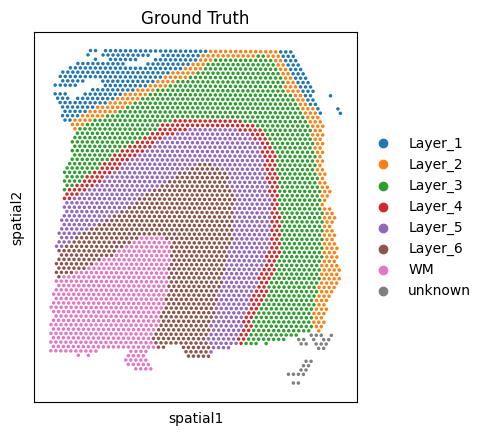
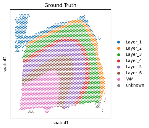
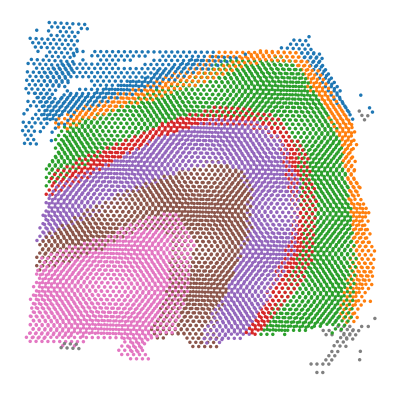
Visualize adata1, adata2, and adata3.

Visualize the spatial distribution of ‘Ground Truth’ annotations for each dataset. This helps in understanding the tissue morphology and layer organization.

[4]:

sc.pl.spatial(adata1, img_key=None, color='Ground Truth')
sc.pl.spatial(adata2, img_key=None, color='Ground Truth')
sc.pl.spatial(adata3, img_key=None, color='Ground Truth')

_images/Tutorial_6_DLPFC_interpolation_8_0.png

_images/Tutorial_6_DLPFC_interpolation_8_1.png

_images/Tutorial_6_DLPFC_interpolation_8_2.png

Align the input datasets adata1 and adata2 using the PASTE2 algorithm.

PASTE2 is used to spatially align two AnnData objects by finding an optimal transformation that minimizes the distance between corresponding spots.

[5]:

from GenOT.utils import PASTE2_align_spatial_data

adata1.obsm['spatial'], adata2.obsm['spatial'] = PASTE2_align_spatial_data(adata1, adata2, visualize=True)

PASTE2 starts...
Starting GLM-PCA...
Iteration: 0 | deviance=4.2825E+6
Iteration: 1 | deviance=4.2825E+6
Iteration: 2 | deviance=4.1865E+6
Iteration: 3 | deviance=4.0313E+6
Iteration: 4 | deviance=3.9559E+6
Iteration: 5 | deviance=3.9226E+6
Iteration: 6 | deviance=3.9048E+6
Iteration: 7 | deviance=3.8942E+6
Iteration: 8 | deviance=3.8876E+6
Iteration: 9 | deviance=3.8831E+6
Iteration: 10 | deviance=3.8797E+6
Iteration: 11 | deviance=3.8769E+6
Iteration: 12 | deviance=3.8747E+6
Iteration: 13 | deviance=3.8728E+6
Iteration: 14 | deviance=3.8712E+6
Iteration: 15 | deviance=3.8699E+6
Iteration: 16 | deviance=3.8687E+6
Iteration: 17 | deviance=3.8677E+6
Iteration: 18 | deviance=3.8668E+6
Iteration: 19 | deviance=3.8660E+6
Iteration: 20 | deviance=3.8653E+6
Iteration: 21 | deviance=3.8647E+6
Iteration: 22 | deviance=3.8641E+6
Iteration: 23 | deviance=3.8636E+6
Iteration: 24 | deviance=3.8631E+6
Iteration: 25 | deviance=3.8626E+6
Iteration: 26 | deviance=3.8622E+6
Iteration: 27 | deviance=3.8618E+6
GLM-PCA finished.
It.  |Loss        |Relative loss|Absolute loss
------------------------------------------------
    0|1.629470e+02|0.000000e+00|0.000000e+00
    1|3.336742e+01|3.883416e+00|1.295796e+02
    2|1.202396e+01|1.775077e+00|2.134346e+01
    3|1.056753e+01|1.378212e-01|1.456430e+00
    4|1.053774e+01|2.827189e-03|2.979219e-02
    5|1.052598e+01|1.117887e-03|1.176685e-02
    6|1.051415e+01|1.124751e-03|1.182580e-02
    7|1.050555e+01|8.188502e-04|8.602469e-03
    8|1.049879e+01|6.437843e-04|6.758955e-03
    9|1.049461e+01|3.979337e-04|4.176159e-03
   10|1.049173e+01|2.742749e-04|2.877619e-03
   11|1.048998e+01|1.667681e-04|1.749395e-03
   12|1.048868e+01|1.242946e-04|1.303686e-03
   13|1.048781e+01|8.350228e-05|8.757556e-04
   14|1.048705e+01|7.169439e-05|7.518629e-04
   15|1.048655e+01|4.810681e-05|5.044744e-04
   16|1.048621e+01|3.218690e-05|3.375186e-04
   17|1.048601e+01|1.956590e-05|2.051682e-04
   18|1.048588e+01|1.186060e-05|1.243688e-04
   19|1.048581e+01|6.549029e-06|6.867190e-05
   20|1.048570e+01|1.094125e-05|1.147266e-04
   21|1.048559e+01|9.945426e-06|1.042837e-04
   22|1.048552e+01|6.964700e-06|7.302851e-05
   23|1.048549e+01|3.334384e-06|3.496264e-05
   24|1.048547e+01|1.783350e-06|1.869926e-05
   25|1.048546e+01|1.107618e-06|1.161388e-05
   26|1.048544e+01|1.171810e-06|1.228695e-05
   27|1.048543e+01|1.719212e-06|1.802667e-05
   28|1.048540e+01|2.407388e-06|2.524242e-05
   29|1.048536e+01|3.734546e-06|3.915807e-05
   30|1.048535e+01|1.443932e-06|1.514013e-05
   31|1.048534e+01|5.351043e-07|5.610751e-06
   32|1.048534e+01|4.176353e-07|4.379047e-06
   33|1.048533e+01|1.684452e-07|1.766204e-06
   34|1.048533e+01|1.453831e-07|1.524390e-06
   35|1.048533e+01|4.463739e-07|4.680376e-06
   36|1.048532e+01|3.445573e-07|3.612796e-06
   37|1.048532e+01|8.397153e-07|8.804680e-06
   38|1.048531e+01|4.483258e-07|4.700835e-06
   39|1.048531e+01|2.094770e-07|2.196431e-06
   40|1.048531e+01|5.465983e-08|5.731251e-07
   41|1.048531e+01|8.697478e-09|9.119574e-08
   42|1.048531e+01|6.659006e-09|6.982173e-08
 1000|1.048531e+01|8.122292e-10|8.516473e-09

_images/Tutorial_6_DLPFC_interpolation_10_1.png

Get unique marker genes from adata3 based on its ‘Ground Truth’ annotations. These marker genes will be used to ensure consistent gene sets across all datasets.

[6]:

from GenOT.utils import get_unique_marker_genes

unique_marker_genes = get_unique_marker_genes(adata3, annotation_column_name='Ground Truth', n_top_genes=10)

Using annotation column 'Ground Truth' for marker gene analysis...
Unique values in annotation column: ['Layer_3', 'Layer_1', 'WM', 'Layer_5', 'Layer_6', 'Layer_2', 'Layer_4', 'unknown']
Extracted 66 unique marker genes from the top 10 genes per annotation group.
First 10 extracted marker genes: ['AGR3', 'ATP1A1', 'AZGP1', 'B3GALT2', 'C11orf87', 'CA10', 'CARTPT', 'CBX6', 'CLDN11', 'CLDND1']...

Data Preprocessing

This section preprocesses the data by ensuring all datasets contain the same set of genes, specifically the marker genes identified earlier.

[7]:

common_genes = set(unique_marker_genes) & set(adata1.var_names) & set(adata2.var_names) & set(adata3.var_names)
matching_genes = list(common_genes)

adata1 = adata1[:, matching_genes].copy()
adata2 = adata2[:, matching_genes].copy()
adata3 = adata3[:, matching_genes].copy()

Run GenOT

This section initializes and trains the GenOT DualEncoder, which learns a shared latent space representation for the input spatial transcriptomics datasets.

[8]:

# define model
Encoder = genot.DualEncoder(adata1, adata2, device=device, pca_n=16)

WARNING: adata.X seems to be already log-transformed.
WARNING: adata.X seems to be already log-transformed.

[9]:

adata1, adata2 = Encoder.train_encoder()

Training DualEncoder on 2 datasets with 700 epochs...

Training: 100%|██████████| 700/700 [00:22<00:00, 31.65it/s]

Training completed!

Compute the spatial barycenter.

[10]:

from GenOT.OTutils import compute_spatial_barycenter

Xb_s, s_transport_plans = compute_spatial_barycenter(adata1, adata2, num_barycenters=adata3.n_obs)

It.  |Loss        |Relative loss|Absolute loss
------------------------------------------------
    0|1.526740e+07|0.000000e+00|0.000000e+00
    1|1.386171e+07|1.014077e-01|1.405685e+06
    2|1.386171e+07|0.000000e+00|0.000000e+00
It.  |Loss        |Relative loss|Absolute loss
------------------------------------------------
    0|1.560258e+07|0.000000e+00|0.000000e+00
    1|1.393915e+07|1.193348e-01|1.663426e+06
    2|1.393915e+07|0.000000e+00|0.000000e+00
It.  |Err
-------------------
    0|1.269066e+07|
    0|1.608939e+05|
It.  |Loss        |Relative loss|Absolute loss
------------------------------------------------
    0|1.315560e+07|0.000000e+00|0.000000e+00
    1|1.751202e+06|6.512327e+00|1.140440e+07
    2|1.735259e+06|9.187614e-03|1.594289e+04
    3|1.733098e+06|1.247302e-03|2.161696e+03
    4|1.733098e+06|0.000000e+00|0.000000e+00
It.  |Loss        |Relative loss|Absolute loss
------------------------------------------------
    0|1.338249e+07|0.000000e+00|0.000000e+00
    1|1.864172e+06|6.178786e+00|1.151832e+07
    2|1.850695e+06|7.282146e-03|1.347703e+04
    3|1.850147e+06|2.964959e-04|5.485609e+02
    4|1.849901e+06|1.328432e-04|2.457467e+02
    5|1.849901e+06|0.000000e+00|0.000000e+00
    1|6.255801e+06|
    1|4.585554e+04|
It.  |Loss        |Relative loss|Absolute loss
------------------------------------------------
    0|1.385275e+07|0.000000e+00|0.000000e+00
    1|5.144138e+04|2.682920e+02|1.380131e+07
    2|2.491653e+04|1.064548e+00|2.652485e+04
    3|2.491579e+04|2.983232e-05|7.432956e-01
    4|2.491512e+04|2.685066e-05|6.689873e-01
    5|2.491499e+04|4.946091e-06|1.232318e-01
It.  |Loss        |Relative loss|Absolute loss
------------------------------------------------
    0|1.403153e+07|0.000000e+00|0.000000e+00
    1|4.188514e+04|3.340003e+02|1.398965e+07
    2|2.517658e+04|6.636546e-01|1.670855e+04
    3|2.517566e+04|3.647349e-05|9.182442e-01
    4|2.517561e+04|2.322090e-06|5.846001e-02
    2|3.023500e+05|
    2|4.879279e+03|
It.  |Loss        |Relative loss|Absolute loss
------------------------------------------------
    0|1.388917e+07|0.000000e+00|0.000000e+00
    1|6.904005e+04|2.001756e+02|1.382013e+07
    2|1.799695e+04|2.836208e+00|5.104310e+04
    3|1.799676e+04|1.082792e-05|1.948675e-01
    4|1.799676e+04|3.308993e-09|5.955114e-05
It.  |Loss        |Relative loss|Absolute loss
------------------------------------------------
    0|1.406795e+07|0.000000e+00|0.000000e+00
    1|5.281460e+04|2.653649e+02|1.401514e+07
    2|1.820903e+04|1.900461e+00|3.460556e+04
    3|1.820878e+04|1.407460e-05|2.562813e-01
    4|1.820878e+04|1.846640e-08|3.362506e-04
    3|5.511423e+04|
    3|9.412721e+02|
It.  |Loss        |Relative loss|Absolute loss
------------------------------------------------
    0|1.388972e+07|0.000000e+00|0.000000e+00
    1|6.805087e+04|2.031079e+02|1.382167e+07
    2|1.764421e+04|2.856839e+00|5.040666e+04
    3|1.764384e+04|2.088678e-05|3.685230e-01
    4|1.764384e+04|3.249027e-08|5.732530e-04
It.  |Loss        |Relative loss|Absolute loss
------------------------------------------------
    0|1.406850e+07|0.000000e+00|0.000000e+00
    1|5.442088e+04|2.575129e+02|1.401408e+07
    2|1.795211e+04|2.031447e+00|3.646877e+04
    3|1.795180e+04|1.764359e-05|3.167342e-01
    4|1.795180e+04|1.418568e-15|2.546585e-11
    4|3.770926e+04|
    4|6.411836e+02|
It.  |Loss        |Relative loss|Absolute loss
------------------------------------------------
    0|1.388990e+07|0.000000e+00|0.000000e+00
    1|6.866108e+04|2.012966e+02|1.382124e+07
    2|1.746666e+04|2.930979e+00|5.119442e+04
    3|1.746637e+04|1.661041e-05|2.901235e-01
    4|1.746637e+04|1.394787e-07|2.436186e-03
It.  |Loss        |Relative loss|Absolute loss
------------------------------------------------
    0|1.406868e+07|0.000000e+00|0.000000e+00
    1|5.194040e+04|2.698620e+02|1.401674e+07
    2|1.780608e+04|1.917004e+00|3.413432e+04
    3|1.780604e+04|1.973525e-06|3.514067e-02
    5|3.067786e+04|
    5|5.162343e+02|
It.  |Loss        |Relative loss|Absolute loss
------------------------------------------------
    0|1.389002e+07|0.000000e+00|0.000000e+00
    1|6.706564e+04|2.061109e+02|1.382296e+07
    2|1.736066e+04|2.863081e+00|4.970498e+04
    3|1.736023e+04|2.463403e-05|4.276526e-01
    4|1.736023e+04|2.511478e-08|4.359985e-04
It.  |Loss        |Relative loss|Absolute loss
------------------------------------------------
    0|1.406880e+07|0.000000e+00|0.000000e+00
    1|5.212078e+04|2.689270e+02|1.401668e+07
    2|1.769896e+04|1.944849e+00|3.442182e+04
    3|1.769848e+04|2.712819e-05|4.801278e-01
    4|1.769848e+04|7.511497e-08|1.329421e-03
    6|2.587306e+04|
    6|4.395153e+02|
It.  |Loss        |Relative loss|Absolute loss
------------------------------------------------
    0|1.389011e+07|0.000000e+00|0.000000e+00
    1|6.686594e+04|2.067307e+02|1.382324e+07
    2|1.727665e+04|2.870307e+00|4.958929e+04
    3|1.727644e+04|1.212775e-05|2.095243e-01
    4|1.727644e+04|1.301304e-09|2.248190e-05
It.  |Loss        |Relative loss|Absolute loss
------------------------------------------------
    0|1.406889e+07|0.000000e+00|0.000000e+00
    1|5.520170e+04|2.538634e+02|1.401369e+07
    2|1.762440e+04|2.132118e+00|3.757730e+04
    3|1.762402e+04|2.151800e-05|3.792336e-01
    4|1.762402e+04|5.608835e-08|9.885023e-04
    7|2.122793e+04|
    7|3.599307e+02|
It.  |Loss        |Relative loss|Absolute loss
------------------------------------------------
    0|1.389017e+07|0.000000e+00|0.000000e+00
    1|6.878399e+04|2.009391e+02|1.382139e+07
    2|1.723114e+04|2.991841e+00|5.155284e+04
    3|1.723068e+04|2.661829e-05|4.586513e-01
    4|1.723068e+04|1.650662e-08|2.844203e-04
It.  |Loss        |Relative loss|Absolute loss
------------------------------------------------
    0|1.406895e+07|0.000000e+00|0.000000e+00
    1|5.388683e+04|2.600833e+02|1.401507e+07
    2|1.756622e+04|2.067640e+00|3.632061e+04
    3|1.756541e+04|4.625594e-05|8.125043e-01
    4|1.756540e+04|2.487714e-07|4.369770e-03
    8|1.793257e+04|
    8|3.004944e+02|
It.  |Loss        |Relative loss|Absolute loss
------------------------------------------------
    0|1.389022e+07|0.000000e+00|0.000000e+00
    1|6.684841e+04|2.067868e+02|1.382337e+07
    2|1.719598e+04|2.887443e+00|4.965242e+04
    3|1.719476e+04|7.100974e-05|1.220996e+00
    4|1.719476e+04|2.335213e-07|4.015342e-03
It.  |Loss        |Relative loss|Absolute loss
------------------------------------------------
    0|1.406900e+07|0.000000e+00|0.000000e+00
    1|5.331611e+04|2.628789e+02|1.401568e+07
    2|1.752571e+04|2.042165e+00|3.579040e+04
    3|1.752557e+04|7.752226e-06|1.358622e-01
    9|1.618058e+04|
    9|2.707699e+02|

Run decoder

Initialize and train the GenOT Decoder. The decoder learns to reconstruct gene expression from the latent space embeddings.

[11]:

decoder = genot.Decoder(
    input_size=adata1.obsm['emb'].shape[1],  # Input dimension
    output_size=adata1.X.shape[1],  # Output dimension
)
# Train the decoder
trained_decoder = decoder.train_decoder(adata1, adata2, decoder, epochs=500, batch_size=2048)

100%|██████████| 500/500 [00:33<00:00, 14.73it/s]

[12]:

# Extract the learned embeddings from adata1 and adata2.
embd0 = adata1.obsm['emb']
embd1 = adata2.obsm['emb']

Compute the embedding barycenter for the latent representations.

[13]:

from GenOT.OTutils import compute_emb_barycenter

Xb, e_transport_plans = compute_emb_barycenter(
    adata1, adata2,
    weight1=0.5,
    alpha=0.5,
    num_barycenters=adata3.n_obs
)

It.  |Loss        |Relative loss|Absolute loss
------------------------------------------------
    0|4.741920e+01|0.000000e+00|0.000000e+00
    1|3.864771e+01|2.269601e-01|8.771488e+00
    2|3.864771e+01|0.000000e+00|0.000000e+00
It.  |Loss        |Relative loss|Absolute loss
------------------------------------------------
    0|3.640727e+01|0.000000e+00|0.000000e+00
    1|2.842808e+01|2.806795e-01|7.979181e+00
    2|2.840253e+01|8.997296e-04|2.555460e-02
    3|2.840253e+01|0.000000e+00|0.000000e+00
It.  |Err
-------------------
    0|7.186842e+03|
    0|4.668437e+02|
It.  |Loss        |Relative loss|Absolute loss
------------------------------------------------
    0|1.402055e+01|0.000000e+00|0.000000e+00
    1|1.855133e+00|6.557708e+00|1.216542e+01
    2|1.846197e+00|4.840139e-03|8.935850e-03
    3|1.846197e+00|0.000000e+00|0.000000e+00
It.  |Loss        |Relative loss|Absolute loss
------------------------------------------------
    0|1.316487e+01|0.000000e+00|0.000000e+00
    1|1.514189e+00|7.694340e+00|1.165068e+01
    2|1.470494e+00|2.971447e-02|4.369494e-02
    3|1.470494e+00|0.000000e+00|0.000000e+00
    1|2.553234e+03|
    1|5.600021e+01|
It.  |Loss        |Relative loss|Absolute loss
------------------------------------------------
    0|1.406848e+01|0.000000e+00|0.000000e+00
    1|9.724391e-01|1.346721e+01|1.309604e+01
    2|9.579550e-01|1.511980e-02|1.448409e-02
    3|9.579550e-01|0.000000e+00|0.000000e+00
It.  |Loss        |Relative loss|Absolute loss
------------------------------------------------
    0|1.349701e+01|0.000000e+00|0.000000e+00
    1|1.055438e+00|1.178807e+01|1.244157e+01
    2|9.762700e-01|8.109177e-02|7.916746e-02
    3|9.762700e-01|0.000000e+00|0.000000e+00
    2|2.584962e+02|
    2|1.200261e+01|
It.  |Loss        |Relative loss|Absolute loss
------------------------------------------------
    0|1.411329e+01|0.000000e+00|0.000000e+00
    1|9.411063e-01|1.399649e+01|1.317219e+01
    2|9.329591e-01|8.732595e-03|8.147155e-03
    3|9.284088e-01|4.901245e-03|4.550359e-03
    4|9.284088e-01|0.000000e+00|0.000000e+00
It.  |Loss        |Relative loss|Absolute loss
------------------------------------------------
    0|1.354182e+01|0.000000e+00|0.000000e+00
    1|1.035858e+00|1.207305e+01|1.250596e+01
    2|9.505066e-01|8.979548e-02|8.535120e-02
    3|9.504068e-01|1.050017e-04|9.979437e-05
    4|9.504068e-01|0.000000e+00|0.000000e+00
    3|1.603657e+02|
    3|7.572746e+00|
It.  |Loss        |Relative loss|Absolute loss
------------------------------------------------
    0|1.412767e+01|0.000000e+00|0.000000e+00
    1|9.264099e-01|1.424991e+01|1.320126e+01
    2|9.173938e-01|9.827951e-03|9.016102e-03
    3|9.173938e-01|0.000000e+00|0.000000e+00
It.  |Loss        |Relative loss|Absolute loss
------------------------------------------------
    0|1.355619e+01|0.000000e+00|0.000000e+00
    1|1.018920e+00|1.230447e+01|1.253727e+01
    2|9.383659e-01|8.584497e-02|8.055399e-02
    3|9.383658e-01|9.151875e-08|8.587807e-08
    4|1.328084e+02|
    4|6.005610e+00|
It.  |Loss        |Relative loss|Absolute loss
------------------------------------------------
    0|1.413600e+01|0.000000e+00|0.000000e+00
    1|9.202902e-01|1.436037e+01|1.321571e+01
    2|9.097421e-01|1.159466e-02|1.054815e-02
    3|9.097421e-01|0.000000e+00|0.000000e+00
It.  |Loss        |Relative loss|Absolute loss
------------------------------------------------
    0|1.356453e+01|0.000000e+00|0.000000e+00
    1|1.015590e+00|1.235630e+01|1.254894e+01
    2|9.305206e-01|9.142149e-02|8.506958e-02
    3|9.305204e-01|1.618941e-07|1.506457e-07
    5|1.236219e+02|
    5|5.707096e+00|
It.  |Loss        |Relative loss|Absolute loss
------------------------------------------------
    0|1.414319e+01|0.000000e+00|0.000000e+00
    1|9.092224e-01|1.455526e+01|1.323396e+01
    2|9.018503e-01|8.174382e-03|7.372069e-03
    3|9.010745e-01|8.609547e-04|7.757843e-04
    4|9.010745e-01|0.000000e+00|0.000000e+00
It.  |Loss        |Relative loss|Absolute loss
------------------------------------------------
    0|1.357171e+01|0.000000e+00|0.000000e+00
    1|9.996367e-01|1.257664e+01|1.257207e+01
    2|9.238908e-01|8.198572e-02|7.574585e-02
    3|9.238907e-01|8.258421e-08|7.629878e-08
    6|1.038752e+02|
    6|4.729515e+00|
It.  |Loss        |Relative loss|Absolute loss
------------------------------------------------
    0|1.414928e+01|0.000000e+00|0.000000e+00
    1|9.025142e-01|1.467763e+01|1.324677e+01
    2|8.962023e-01|7.042916e-03|6.311878e-03
    3|8.962023e-01|0.000000e+00|0.000000e+00
It.  |Loss        |Relative loss|Absolute loss
------------------------------------------------
    0|1.357780e+01|0.000000e+00|0.000000e+00
    1|9.924141e-01|1.268159e+01|1.258539e+01
    2|9.177212e-01|8.138959e-02|7.469295e-02
    3|9.177211e-01|6.514683e-08|5.978662e-08
    7|1.004071e+02|
    7|4.477300e+00|
It.  |Loss        |Relative loss|Absolute loss
------------------------------------------------
    0|1.415446e+01|0.000000e+00|0.000000e+00
    1|8.970260e-01|1.477932e+01|1.325743e+01
    2|8.931338e-01|4.357849e-03|3.892142e-03
    3|8.931338e-01|0.000000e+00|0.000000e+00
It.  |Loss        |Relative loss|Absolute loss
------------------------------------------------
    0|1.358298e+01|0.000000e+00|0.000000e+00
    1|9.911492e-01|1.270428e+01|1.259183e+01
    2|9.114000e-01|8.750175e-02|7.974910e-02
    3|9.114000e-01|1.066095e-07|9.716392e-08
    8|9.807398e+01|
    8|4.318798e+00|
It.  |Loss        |Relative loss|Absolute loss
------------------------------------------------
    0|1.415895e+01|0.000000e+00|0.000000e+00
    1|8.926285e-01|1.486208e+01|1.326632e+01
    2|8.882007e-01|4.985114e-03|4.427782e-03
    3|8.881973e-01|3.886970e-06|3.452396e-06
It.  |Loss        |Relative loss|Absolute loss
------------------------------------------------
    0|1.358747e+01|0.000000e+00|0.000000e+00
    1|9.849741e-01|1.279475e+01|1.260250e+01
    2|9.074867e-01|8.538674e-02|7.748734e-02
    3|9.074867e-01|3.718391e-08|3.374390e-08
    9|8.044219e+01|
    9|3.651166e+00|

Since the spatial barycenter and embedding barycenter reside in different spaces (not one-to-one cell correspondences), we align them by constraining the embedding barycenter. Refer to the [update_embedding_barycenter] function for details.

[14]:

from GenOT.OTutils import update_embedding_barycenter

Xb = update_embedding_barycenter(Xb_s, Xb, s_transport_plans, e_transport_plans)

Use the trained decoder to transform the embedding barycenter into gene expression values.

[15]:

new_embedding = torch.tensor(Xb, dtype=torch.float32)
new_embedding = new_embedding.to("cuda" if torch.cuda.is_available() else "cpu")

trained_decoder.eval()
with torch.no_grad():
    reconstructed_features = trained_decoder(new_embedding)

reconstructed_gene_expression = reconstructed_features.cpu().numpy()

print("Reconstructed Features Shape:", reconstructed_gene_expression.shape)

Reconstructed Features Shape: (3673, 66)

Create a new adata object where the gene expression matrix equals the generated expression values, and spatial coordinates match the spatial barycenter.

[16]:

new_adata = adata3.copy()
X = reconstructed_gene_expression.copy()
thresholds = X.max(axis=0) / 2
for i, threshold in enumerate(thresholds):
    X[:, i][X[:, i] < threshold] = 0
new_adata.X = X
new_adata.obsm['spatial'] = Xb_s

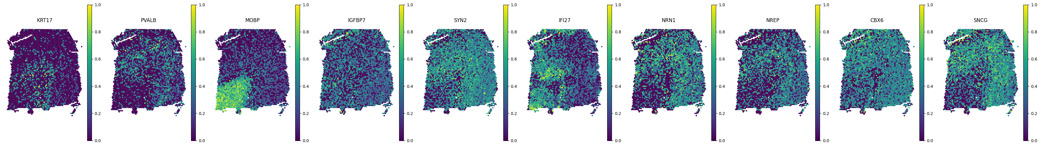
Map the generated gene expression data to the target dataset using the [create_mapped_adata] function.

[17]:

from GenOT.OTutils import create_mapped_adata

mapped_adata = create_mapped_adata(new_adata, adata3, threshold_denominator=2)

[18]:

import matplotlib.pyplot as plt
import scanpy as sc

import random

genes_of_interest = list(common_genes)[:10]

fig, axes = plt.subplots(1, 10, figsize=(35, 5))
plt.subplots_adjust(wspace=0.3)

for i, gene in enumerate(genes_of_interest):
    sc.pl.spatial(
        new_adata,
        color=gene,
        ax=axes[i],
        title=gene,
        show=False,
        size=1.5,
        spot_size=100,
        cmap='viridis',
        frameon=False,
        img_key=None
    )

plt.tight_layout()
plt.show()

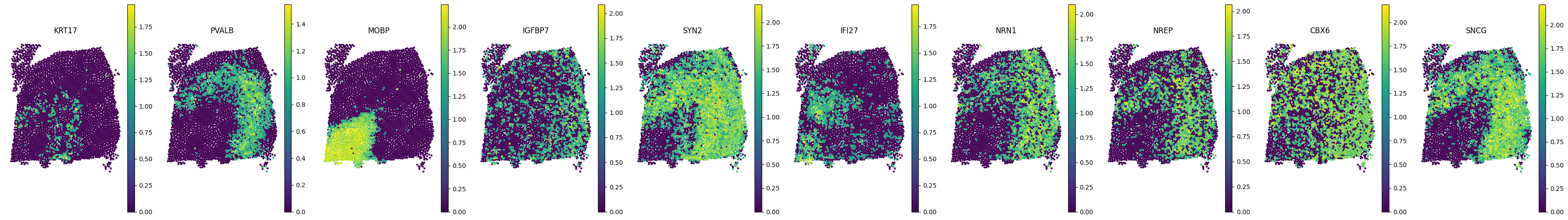
_images/Tutorial_6_DLPFC_interpolation_35_0.png

Visualize the mapped data, original datasets (adata1/151673 and adata2/151675), and the imputed dataset (adata3/151674)

[19]:

import matplotlib.pyplot as plt
import scanpy as sc

import random

genes_of_interest = list(common_genes)[:10]

fig, axes = plt.subplots(1, 10, figsize=(35, 5))
plt.subplots_adjust(wspace=0.3)

for i, gene in enumerate(genes_of_interest):
    sc.pl.spatial(
        mapped_adata,
        color=gene,
        ax=axes[i],
        title=gene,
        show=False,
        size=1.5,
        spot_size=100,
        cmap='viridis',
        frameon=False
    )

plt.tight_layout()
plt.show()

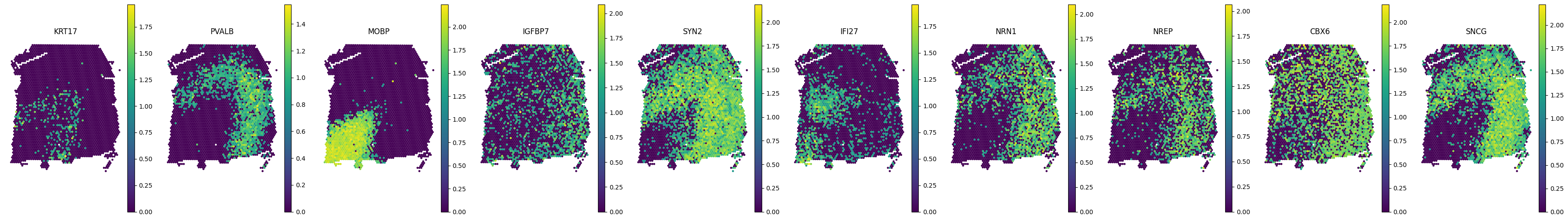
_images/Tutorial_6_DLPFC_interpolation_37_0.png

[20]:

fig, axes = plt.subplots(1, 10, figsize=(35, 5))
plt.subplots_adjust(wspace=0.3)

for i, gene in enumerate(genes_of_interest):
    sc.pl.spatial(
        adata1,
        color=gene,
        ax=axes[i],
        img_key=None,
        title=gene,
        show=False,
        size=1.5,
        spot_size=100,
        cmap='viridis',
        frameon=False
    )

plt.tight_layout()
plt.show()

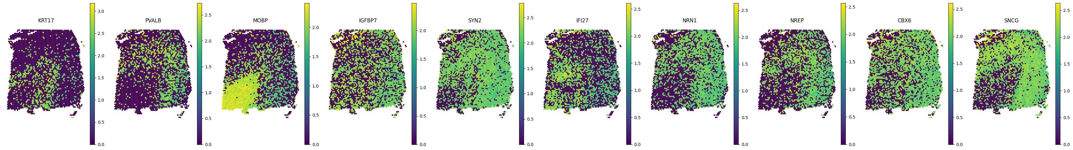
_images/Tutorial_6_DLPFC_interpolation_38_0.png

[21]:

fig, axes = plt.subplots(1, 10, figsize=(35, 5))
plt.subplots_adjust(wspace=0.3)

for i, gene in enumerate(genes_of_interest):
    sc.pl.spatial(
        adata2,
        color=gene,
        img_key=None,
        ax=axes[i],
        show=False,
        size=1.5,
        spot_size=100,
        cmap='viridis',
        frameon=False
    )

plt.tight_layout()
plt.show()

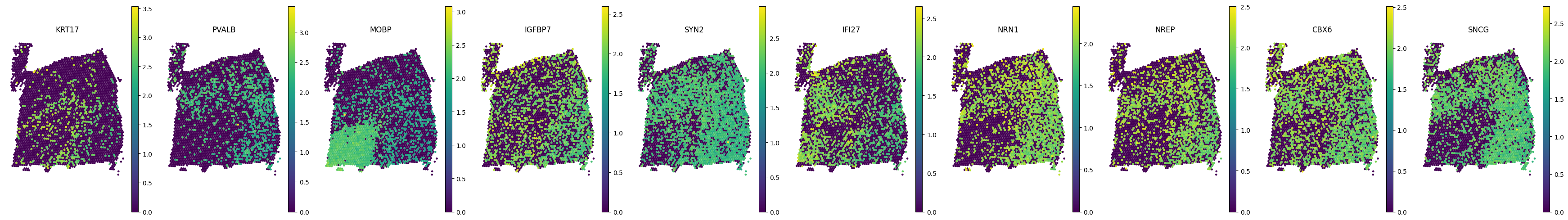
_images/Tutorial_6_DLPFC_interpolation_39_0.png

[22]:

fig, axes = plt.subplots(1, 10, figsize=(35, 5))
plt.subplots_adjust(wspace=0.3)

for i, gene in enumerate(genes_of_interest):
    sc.pl.spatial(
        adata3,
        img_key=None,
        color=gene,
        ax=axes[i],
        title=gene,
        show=False,
        size=1.5,
        spot_size=100,
        cmap='viridis',
        frameon=False
    )

plt.tight_layout()
plt.show()

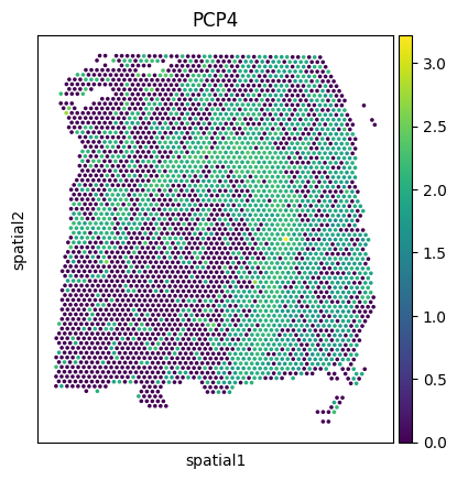
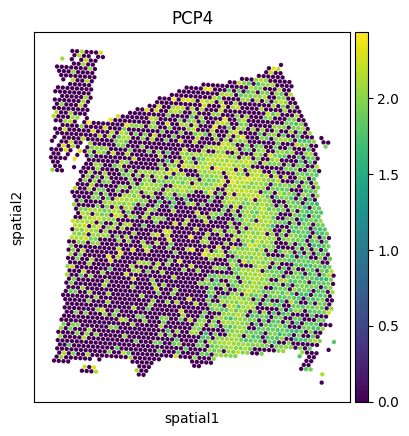
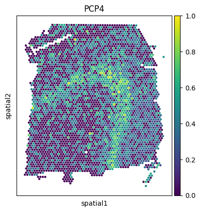
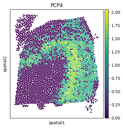
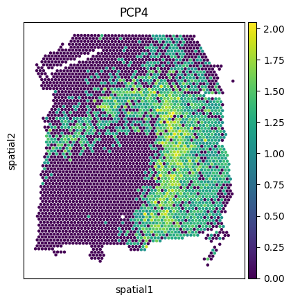
_images/Tutorial_6_DLPFC_interpolation_40_0.png

Visualize the PCP4 gene expression across datasets.

[23]:

sc.pl.spatial(adata1, img_key=None, color='PCP4', cmap='viridis', size=2, spot_size=50)
sc.pl.spatial(adata2, img_key=None, color='PCP4', cmap='viridis', size=2.5, spot_size=50)
sc.pl.spatial(adata3, img_key=None, color='PCP4', cmap='viridis', size=2.5, spot_size=50)
sc.pl.spatial(new_adata, img_key=None, color='PCP4', cmap='viridis', size=2.5, spot_size=50)
sc.pl.spatial(mapped_adata, img_key=None, color='PCP4', cmap='viridis', size=2.5, spot_size=50)

_images/Tutorial_6_DLPFC_interpolation_42_0.png

_images/Tutorial_6_DLPFC_interpolation_42_1.png

_images/Tutorial_6_DLPFC_interpolation_42_2.png

_images/Tutorial_6_DLPFC_interpolation_42_3.png

_images/Tutorial_6_DLPFC_interpolation_42_4.png

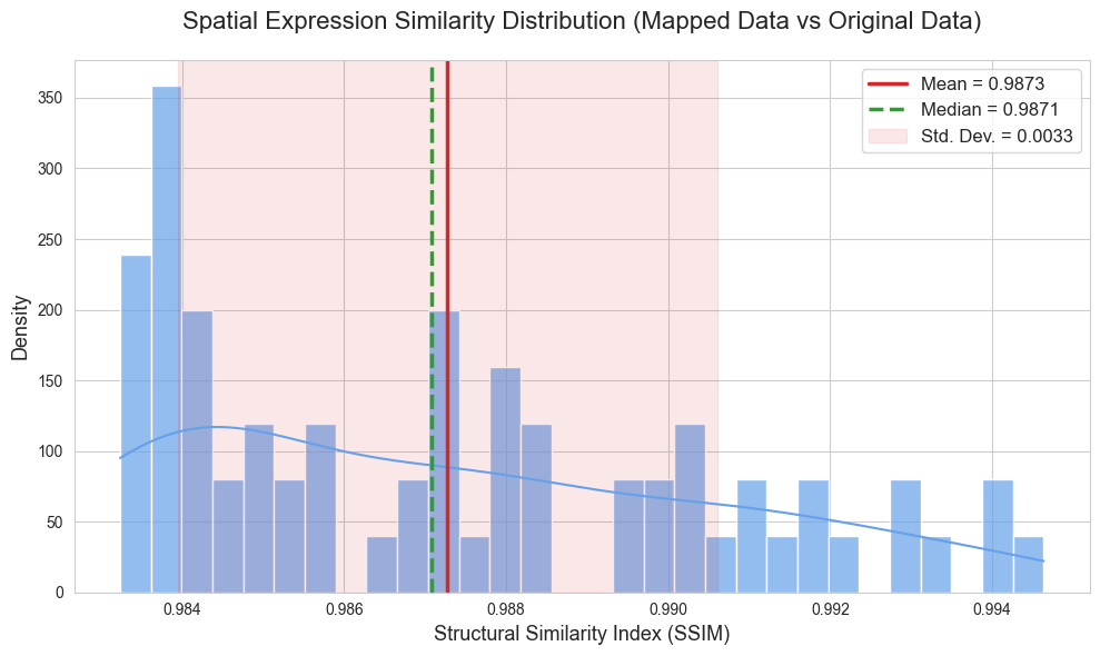
[24]:

from GenOT.plotting import compare_spatial_expression_all_genes
# Compare the spatial expression patterns between the mapped (imputed) data and the original target data.
# This function calculates and plots similarity metrics (e.g., SSIM) for all genes.
mean_ssim, scores_df = compare_spatial_expression_all_genes(
    adata1=mapped_adata,
    adata1_name="Mapped Data",
    adata2=adata3,
    adata2_name="Original Data",
    max_genes=None,
    output_csv=None,
    plot_file=None,
    figsize=(10, 6)
)

Starting comparison for 66 common genes...

Calculating gene SSIM scores: 100%|██████████| 66/66 [01:02<00:00,  1.05it/s]


==================================================
Analysis complete! Processed 66 genes
Mean SSIM: 0.9873 ± 0.0033
Median SSIM: 0.9871
==================================================

_images/Tutorial_6_DLPFC_interpolation_43_3.png

[25]:

from GenOT.plotting import calculate_gene_embedding_metrics, plot_gene_embedding_metrics_distributions
# Calculate various metrics to evaluate the quality of the gene embeddings derived from the imputation.
# These metrics assess how well the imputed gene expression preserves the original's gene-embedding relationships.
df = calculate_gene_embedding_metrics(adata3, mapped_adata, n_pca_components=16)
# Plot the distributions of these calculated gene embedding metrics.
plot_gene_embedding_metrics_distributions(df)

--- Starting gene embedding metric calculation ---
Original adata shape: (3673, 66)
Original mapped_adata shape: (3673, 66)
Transposed adata_g1 shape (genes x cells): (66, 3673)
Transposed adata_g2 shape (genes x cells): (66, 3673)
Found 66 common genes for analysis.
adata_g1 shape after common gene filtering: (66, 3673)
adata_g2 shape after common gene filtering: (66, 3673)

Performing PCA (16 dimensions) for both datasets...
Gene embedding dimensions for Dataset 1: (66, 16)
Gene embedding dimensions for Dataset 2: (66, 16)

Calculating similarity metrics: PCC, Cosine Similarity, RMSE, JS Divergence...

--- Metric calculation complete ---

--- Generating distribution plots for similarity metrics ---
Average PCC: 0.5518
Average Cosine Similarity: 0.5618
Average RMSE: 9.7619
Average JS Divergence: 0.4180

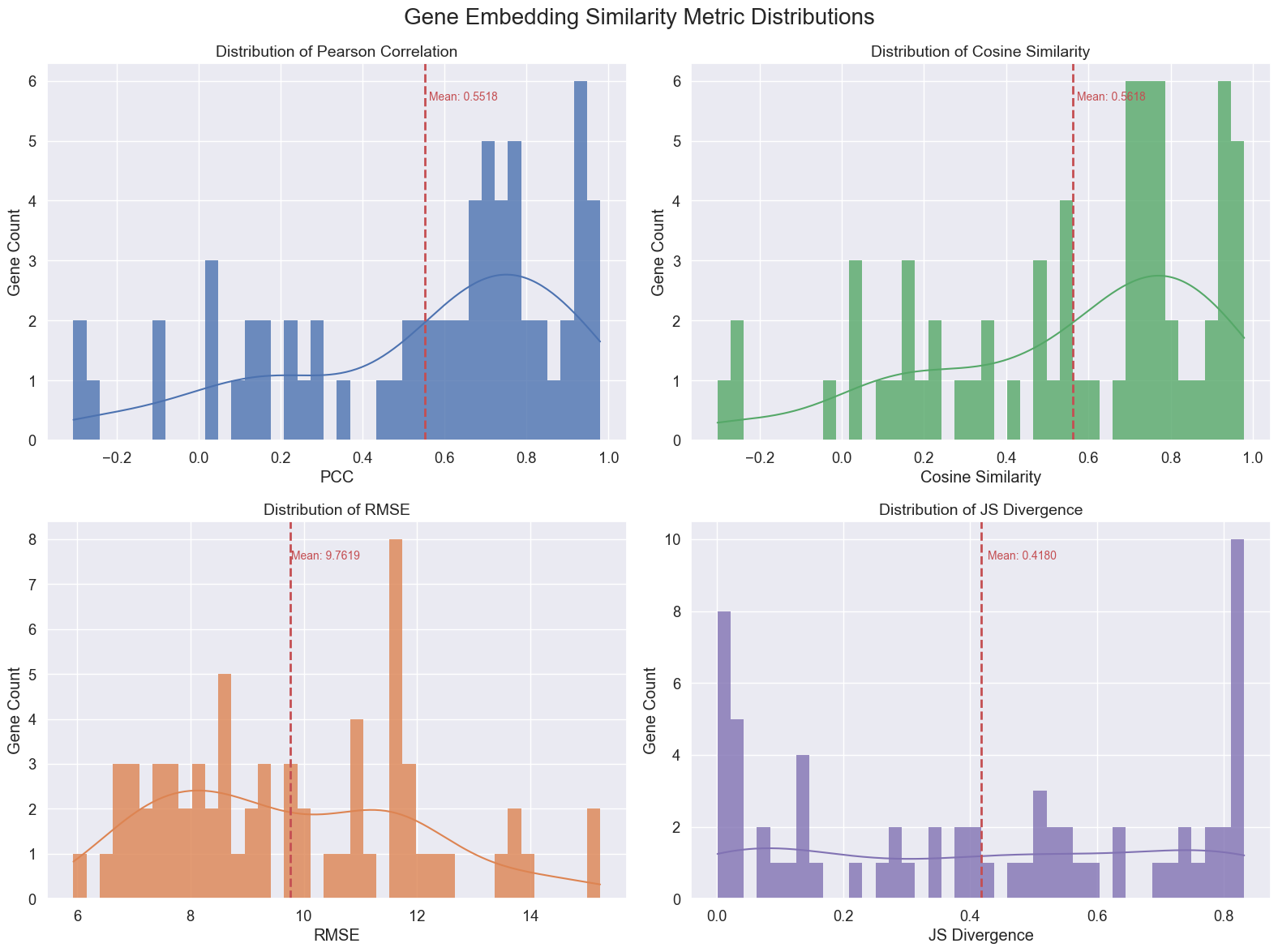
_images/Tutorial_6_DLPFC_interpolation_44_1.png


--- Visualization complete ---

[25]:

[25]:

[25]: